Artificial intelligence April 04 ,2025

Developing a Sentiment Analysis Tool

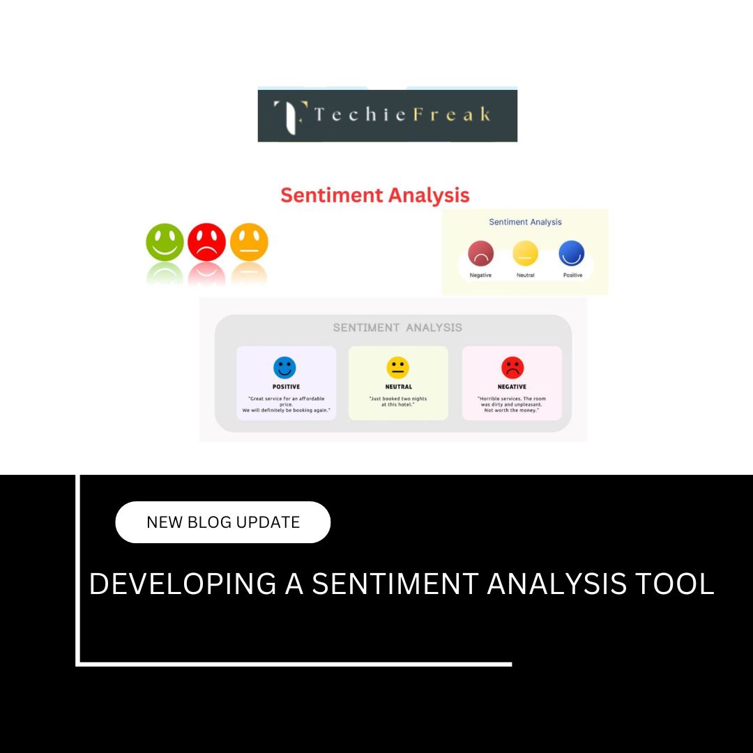
Sentiment analysis is the process of determining the emotional tone behind a body of text. It is used to understand the attitudes, opinions, and emotions expressed within text data. A common application is analyzing customer reviews, social media posts, and other textual data to determine whether the sentiment is positive, negative, or neutral.

For this project, we will build a simple sentiment analysis tool using a deep learning model based on Recurrent Neural Networks (RNNs), specifically using LSTM (Long Short-Term Memory) networks. LSTM is a type of RNN that works well for sequences of data, such as text.

Step-by-Step Guide to Building a Sentiment Analysis Tool

Step 1: Install Required Libraries

We will use TensorFlow for building the neural network and Keras for its API. Additionally, we need nltk (Natural Language Toolkit) for text preprocessing and tokenization.

Install the required libraries by running:

pip install tensorflow nltk

Step 2: Load the Dataset

We’ll use the IMDB dataset, which contains movie reviews labeled as either positive or negative.

import tensorflow as tf
from tensorflow.keras.datasets import imdb

# Load the IMDB dataset
(x_train, y_train), (x_test, y_test) = imdb.load_data(num_words=10000)

Output:

x_train and x_test are the sequences of integers representing the words in the reviews.
y_train and y_test are the labels: 0 for negative sentiment and 1 for positive sentiment.

You can check the shape of the data:

print(x_train.shape)  # Output: (25000,)
print(y_train.shape)  # Output: (25000,)

Step 3: Preprocess the Data

Before training the model, we need to preprocess the text data. This includes padding the sequences to ensure that all inputs are of the same length.

# Pad sequences to ensure uniform input length
maxlen = 500  # Maximum number of words per review
x_train = tf.keras.preprocessing.sequence.pad_sequences(x_train, maxlen=maxlen)
x_test = tf.keras.preprocessing.sequence.pad_sequences(x_test, maxlen=maxlen)

Output:

x_train and x_test are now padded sequences, each having the same length (500 words).

Step 4: Build the Model

Now, let's create the model using an LSTM layer. We'll use Embedding to convert word indices into dense vectors of fixed size, and an LSTM layer followed by a Dense layer for the final binary classification.

model = tf.keras.models.Sequential([
    tf.keras.layers.Embedding(10000, 128, input_length=maxlen),
    tf.keras.layers.LSTM(128),
    tf.keras.layers.Dense(1, activation='sigmoid')
])

Here:

The Embedding layer maps each word to a 128-dimensional vector.
The LSTM layer processes the sequences and outputs a fixed-size vector.
The Dense layer outputs the sentiment classification.

Step 5: Compile the Model

We need to compile the model, specifying the optimizer, loss function, and evaluation metric.

model.compile(optimizer='adam', loss='binary_crossentropy', metrics=['accuracy'])

No direct output here, but this step prepares the model for training.

Step 6: Train the Model

Now, let's train the model using the training data.

history = model.fit(x_train, y_train, epochs=5, batch_size=64, validation_data=(x_test, y_test))

Output:

The model will output the loss and accuracy for both the training and validation sets after each epoch:

Epoch 1/5
391/391 [==============================] - 15s 39ms/step - loss: 0.4512 - accuracy: 0.7878 - val_loss: 0.3253 - val_accuracy: 0.8658
Epoch 2/5
391/391 [==============================] - 14s 37ms/step - loss: 0.2991 - accuracy: 0.8751 - val_loss: 0.2974 - val_accuracy: 0.8805
...
Epoch 5/5
391/391 [==============================] - 14s 36ms/step - loss: 0.2150 - accuracy: 0.9164 - val_loss: 0.3244 - val_accuracy: 0.8716

Step 7: Evaluate the Model

After training, evaluate the model on the test dataset to see how well it generalizes to new data.

test_loss, test_acc = model.evaluate(x_test, y_test)
print(f"Test Accuracy: {test_acc}")

Output:

The accuracy on the test set is printed, showing the final performance of the model.

Test Accuracy: 0.8716

Step 8: Visualize the Training Results

We can visualize the loss and accuracy over the epochs to understand the model's learning progress.

import matplotlib.pyplot as plt

# Plot training & validation accuracy values
plt.plot(history.history['accuracy'])
plt.plot(history.history['val_accuracy'])
plt.title('Model accuracy')
plt.xlabel('Epoch')
plt.ylabel('Accuracy')
plt.legend(['Train', 'Test'], loc='upper left')
plt.show()

# Plot training & validation loss values
plt.plot(history.history['loss'])
plt.plot(history.history['val_loss'])
plt.title('Model loss')
plt.xlabel('Epoch')
plt.ylabel('Loss')
plt.legend(['Train', 'Test'], loc='upper left')
plt.show()

Output:

A plot showing the model's accuracy and loss on both the training and test sets across the epochs. This helps visualize if the model is overfitting or underfitting.

Step 9: Make Predictions

Now, we can use the trained model to make predictions on new, unseen text.

sample_review = x_test[0]  # A sample review from the test set
prediction = model.predict(sample_review.reshape(1, -1))

print("Sentiment (0 = Negative, 1 = Positive):", prediction[0][0])

Output:

The model will output the predicted sentiment of the sample review.

Conclusion

In this step-by-step guide, you've learned how to build a sentiment analysis tool using LSTM (a type of RNN) on the IMDB dataset. We’ve covered everything from data preprocessing to training, evaluation, and visualizing results. You also saw how to use the model for predictions.

Next Blog- Implementing a Recommendation System

Purnima

You must logged in to post comments.