Deep Reinforcement Learning: A Comprehensive Guide to Deep Q-Networks (DQN)

1. Introduction to Deep Q-Networks (DQN)

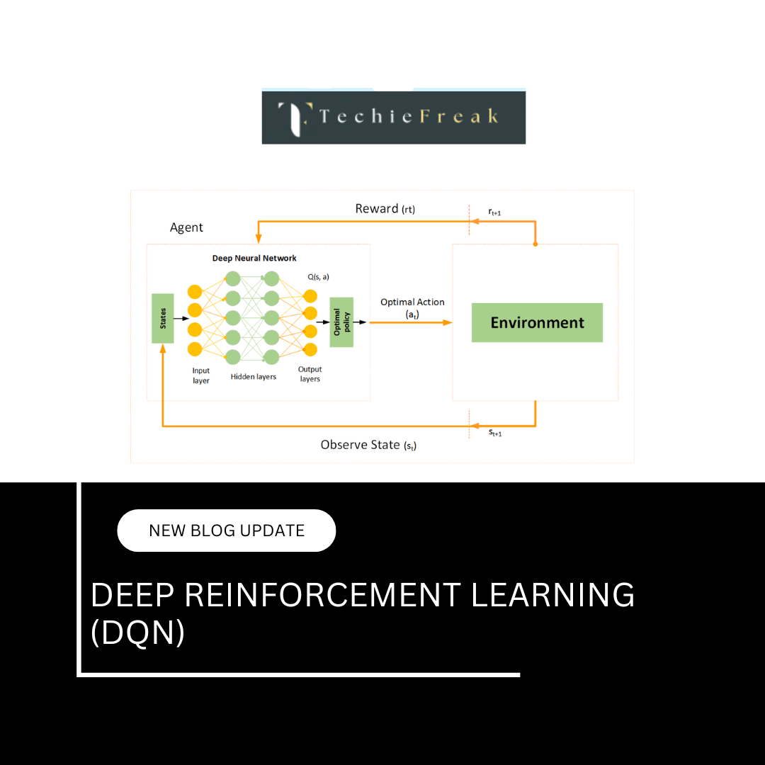
Deep Q-Networks (DQN) mark a significant advancement in Deep Reinforcement Learning (DRL). Developed by DeepMind in 2015, DQN combines traditional Q-learning with deep neural networks (DNNs) to handle complex, high-dimensional environments.

Unlike traditional Q-learning, which struggles with large state-action spaces, DQN can learn directly from raw sensory input, such as images, making it highly effective in Atari games, robotics, and autonomous navigation.

2. The Fundamentals of Q-Learning

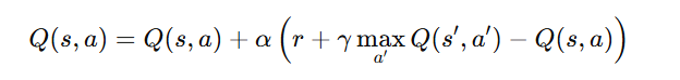
DQN is built upon the foundation of Q-learning, a model-free reinforcement learning algorithm that learns an optimal Q-function:

Key Parameters:

• Q(s, a): Expected reward for taking action aa in state s.
• α: Learning rate (how much new information overrides old information).
• γ: Discount factor (determines the importance of future rewards).
• r: Immediate reward for taking action a.
• s′: Next state.
• a′: Next action.

Limitations of Traditional Q-Learning:

1. Inefficiency in Large State Spaces:
   • Storing a Q-table for all state-action pairs is infeasible in complex environments.
2. Correlated Learning Samples:
   • Consecutive training updates introduce correlations, making learning unstable.
3. Non-stationary Targets:
   • As Q-values update, target values shift, making convergence difficult.

3. How DQN Overcomes Q-Learning’s Limitations

DQN enhances traditional Q-learning by integrating deep learning techniques, solving large-scale reinforcement learning problems efficiently.

Key Innovations in DQN:

1. Deep Neural Networks as Function Approximators
   • Instead of storing Q-values in a table, DQN trains a deep neural network (DNN) to approximate Q(s, a).
   • The input is the state s, and the output is Q-values for all possible actions.
2. Experience Replay (Memory Buffer)
   • Stores past experiences (s, a,r,s′) in a replay buffer.
   • Randomly samples mini-batches for training to reduce correlations.
   • Helps the network learn more stable Q-values.
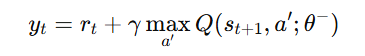
3. Target Network for Stable Learning
   • Maintains a separate target network with weights θ−.
   • Updates the target network periodically rather than at every step, preventing diverging Q-values.

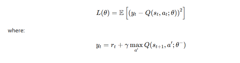
DQN Loss Function

DQN minimizes the error between the predicted Q-value and the target Q-value:

4. The Deep Q-Network Algorithm

Step-by-Step Breakdown

1. Initialize
   • A deep Q-network Q(s, a;θ) with random weights.
   • A target network Q(s, a;θ−)(initially identical to the main network).
   • An experience replay buffer.
2. For each episode:
   • Observe the initial state s0\.
   • Repeat for each time step tt:
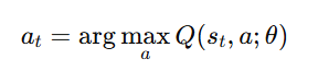
     1. Select action at using ε-greedy policy:
        • With probability ϵ, select a random action (exploration).

        • Otherwise, choose the best action:

          

     2. Execute action at, observe reward rt, and new state st+1.
     3. Store experience (st,at, rt,st+1) in replay buffer.

     4. Sample a mini-batch from the buffer and compute the target Q-values:

        

     5. Update the DQN model by minimizing the loss function.
     6. Periodically update target network weights: θ−=θ
3. Repeat until convergence.

5. Enhancements to DQN

1. Double Deep Q-Networks (DDQN)

• Problem with DQN: Standard Deep Q-Networks (DQN) tend to overestimate Q-values. This happens because the same network is used both for selecting actions and evaluating their Q-values, leading to an optimistic bias that can cause unstable learning.
• Solution in DDQN: It uses two separate networks:
  1. Main (Online) Network – Selects the best action based on learned Q-values.
  2. Target Network – Evaluates the Q-value of that selected action.

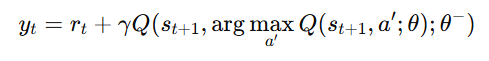
• Prevents over-optimistic value estimates.

2. Dueling DQN

• Issue with Regular DQN: In some states, the choice of action doesn’t matter much (e.g., waiting in a traffic light in a self-driving car). Standard DQNs still calculate Q-values for all actions, which is inefficient.
• Solution in Dueling DQN: It separates the state-value from the advantage of actions:
  • State-value function: Measures how good it is to be in a certain state.
  • Advantage function: Measures how much better a particular action is compared to the average.

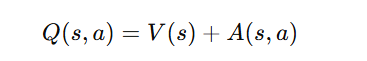
• Helps distinguish between valuable states and optimal actions, improving training.

3. Prioritized Experience Replay

• Issue with Standard Experience Replay:
  • In normal experience replay, we randomly sample past experiences, but not all experiences are equally useful for learning.
• Solution with PER:
  • Instead of random sampling, we prioritize experiences that have higher TD-error (difference between predicted and actual Q-values).
  • TD-error is a signal for how much the model can still learn from a transition.
• Mathematical Concept:
  • Assign priority to each experience based on its absolute TD-error:

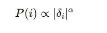
• Use stochastic sampling (not purely greedy) to ensure exploration.
• Why It Works:
  • Focuses on important experiences (high error).
  • Leads to faster convergence.
  • Helps the agent learn from rare but critical transitions.

6. Applications of DQN

1. Gaming

• Atari Games: DQN achieved superhuman performance in games like Pong and Breakout.
• Chess & Go: Variants like AlphaGo used DQN for strategic decision-making.

2. Robotics

• Autonomous Navigation: Robots learn to move efficiently.
• Dexterous Manipulation: DQN-based robotic arms master complex tasks.

3. Autonomous Vehicles

• Path Planning: Self-driving cars optimize safe, efficient routes.
• Traffic Management: AI-driven policies reduce congestion.

4. Finance

• Algorithmic Trading: AI adapts to market trends and optimizes trade execution.
• Portfolio Optimization: Balances risk vs. reward using reinforcement learning.

7. Implementation: Deep Q-Network in Python (TensorFlow/PyTorch)

Here’s a simplified DQN implementation using PyTorch:

import torch
import torch.nn as nn
import torch.optim as optim
import random
import numpy as np
import gym
from collections import deque
# Define DQN Network
class DQN(nn.Module):
   def __init__(self, state_dim, action_dim):
       super(DQN, self).__init__()
       self.fc1 = nn.Linear(state_dim, 128)
       self.fc2 = nn.Linear(128, 128)
       self.fc3 = nn.Linear(128, action_dim)
   
   def forward(self, x):
       x = torch.relu(self.fc1(x))
       x = torch.relu(self.fc2(x))
       return self.fc3(x)
# Hyperparameters
gamma = 0.99  # Discount factor
epsilon = 1.0  # Exploration rate
epsilon_min = 0.01
epsilon_decay = 0.995
lr = 0.001
batch_size = 64
memory_size = 10000
target_update = 10  # Frequency of updating target network
episodes = 500
# Initialize environment
env = gym.make("CartPole-v1")
state_dim = env.observation_space.shape[0]
action_dim = env.action_space.n
# Initialize networks and memory
dqn = DQN(state_dim, action_dim)
target_dqn = DQN(state_dim, action_dim)
target_dqn.load_state_dict(dqn.state_dict())  # Copy weights
optimizer = optim.Adam(dqn.parameters(), lr=lr)
memory = deque(maxlen=memory_size)
def select_action(state, epsilon):
   if random.random() < epsilon:
       return env.action_space.sample()  # Explore
   else:
       state = torch.FloatTensor(state).unsqueeze(0)
       with torch.no_grad():
           return dqn(state).argmax().item()  # Exploit
def train():
   if len(memory) < batch_size:
       return
   batch = random.sample(memory, batch_size)
   states, actions, rewards, next_states, dones = zip(*batch)
   
   states = torch.FloatTensor(states)
   actions = torch.LongTensor(actions).unsqueeze(1)
   rewards = torch.FloatTensor(rewards)
   next_states = torch.FloatTensor(next_states)
   dones = torch.FloatTensor(dones)
   
   q_values = dqn(states).gather(1, actions).squeeze()
   with torch.no_grad():
       next_q_values = target_dqn(next_states).max(1)[0]
       target_q_values = rewards + gamma * next_q_values * (1 - dones)
   
   loss = nn.MSELoss()(q_values, target_q_values)
   optimizer.zero_grad()
   loss.backward()
   optimizer.step()
# Training loop
for episode in range(episodes):
   state = env.reset()
   state = state[0]  # Unwrap state
   total_reward = 0
   done = False
   
   while not done:
       action = select_action(state, epsilon)
       next_state, reward, done, _, _ = env.step(action)
       memory.append((state, action, reward, next_state, done))
       state = next_state
       total_reward += reward
       train()
   
   # Decay epsilon
   epsilon = max(epsilon_min, epsilon * epsilon_decay)
   
   # Update target network
   if episode % target_update == 0:
       target_dqn.load_state_dict(dqn.state_dict())
   
   print(f"Episode {episode+1}, Reward: {total_reward}, Epsilon: {epsilon:.4f}")
env.close()

Explanation of Key Components

1. DQN Network
   • A simple 3-layer neural network to approximate Q-values for given states.
2. Experience Replay (Deque Memory)
   • Stores past experiences and samples them randomly to break the correlation in training data.
3. Epsilon-Greedy Exploration
   • Starts with high exploration (ϵ=1.0\epsilon = 1.0ϵ=1.0) and decays over time to shift towards exploitation.
4. Target Network
   • Updated every 10 episodes to stabilize training and prevent frequent weight changes.
5. Training Loop
   • Runs for 500 episodes, interacting with the environment and learning from experience.

Expected Output

During training, you'll see episode rewards improving as the model learns:

Episode 1, Reward: 12, Epsilon: 0.9950 
Episode 10, Reward: 20, Epsilon: 0.9044
Episode 50, Reward: 150, Epsilon: 0.3660 
Episode 100, Reward: 200, Epsilon: 0.1353 
... 
Episode 500, Reward: 500, Epsilon: 0.0100

8. Conclusion

Deep Q-Networks (DQN) have transformed reinforcement learning by enabling AI to learn from high-dimensional environments. With enhancements like DDQN, Dueling DQN, and Prioritized Experience Replay, DQN remains a foundational algorithm in modern AI research and applications.

Next Blog- Deep Reinforcement Learning (PPO)