A Deep Dive into Calculus for AI: From Derivatives to Optimization

Why Calculus is Crucial for AI and Machine Learning?

Calculus plays a vital role in artificial intelligence (AI) and machine learning (ML) because it provides the mathematical framework needed to understand and optimize models. Machine learning algorithms rely on continuous functions, and calculus helps analyze how these functions change, optimize parameters, and reduce errors in models.

Let’s break it down with key concepts:

1.  Calculus uses in models

When training a machine learning model, we aim to adjust the model’s parameters (weights and biases) to minimize errors. This is done using a function called the loss function, which measures how far the model’s predictions are from the actual values.

• Calculus helps by finding the minimum of this loss function (which means finding the best possible values for weights and biases).
• This is achieved using differentiation, which tells us how the loss changes with respect to each parameter.

For example, in linear regression, we try to find the best-fit line for a dataset. The equation for a line is:

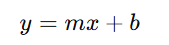
Here, m (slope) and b (intercept) are the parameters we need to adjust to minimize the error.

The loss function (e.g., mean squared error) is differentiated to find the optimal values of m and b, helping the model learn the best fit.

2. Optimization in AI Using Calculus

Optimization is the process of improving model performance by minimizing or maximizing certain functions. In machine learning, we often use gradient-based optimization techniques, such as gradient descent, to find the best parameters.

• Gradient Descent is an iterative method where the algorithm takes small steps in the direction of the steepest descent (negative gradient) to minimize the loss function.
• The gradient (which is a derivative) tells us the slope of the function, helping the model adjust parameters efficiently.

Mathematically, gradient descent updates parameters using the formula:

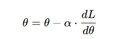
where:

• θ represents the parameter (weight or bias) being updated,
• α is the learning rate,
• dL/dθ is the derivative of the loss function (gradient).

Without calculus, gradient descent and other optimization techniques wouldn’t work, making it impossible for models to learn effectively.

3. Backpropagation in Neural Networks

In deep learning, neural networks learn by adjusting weights through a process called backpropagation.

• Backpropagation uses calculus (chain rule of differentiation) to calculate how much each weight contributed to the overall error.
• It then updates the weights to reduce the error, making the model more accurate over time.

How Backpropagation Works:

1. The input passes through the neural network, producing an output.
2. The error (difference between predicted and actual value) is calculated using a loss function.
3. Using differentiation (gradients), the error is propagated backward to adjust the weights, reducing future errors.

Mathematically, this involves calculating partial derivatives at each layer of the network using the chain rule:

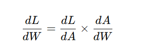
where:

• L is the loss function,
• A is the activation function,
• W represents weights.

Without backpropagation (which is driven by calculus), neural networks would not be able to learn, making deep learning impossible.

More Information-Calculus for AI (Derivatives, Gradients, and Optimization)
 

Understanding Derivatives and Their Role in AI Models

A derivative measures the rate of change of a function with respect to an input variable. In AI and machine learning, derivatives are used to determine how model parameters (such as weights and biases) should be updated to improve performance. They help models learn by minimizing errors and optimizing functions efficiently.

Key Concepts of Derivatives in AI

1. First-Order Derivative

The first-order derivative of a function tells us how the function changes at a specific point. It gives the slope of the function, showing the direction and rate of change.

📌 Application in AI:

• In gradient descent, the first-order derivative (gradient) helps determine the direction in which model parameters should be adjusted to minimize errors.

For example, if we have a loss function L(w) that depends on a weight parameter w, the derivative dL/dw tells us how much the loss will change if we adjust w.

2. Partial Derivatives

When dealing with functions of multiple variables, such as in machine learning models and neural networks, we use partial derivatives to measure the rate of change with respect to each individual variable.

📌 Application in AI:

• Neural networks use partial derivatives to adjust weights for multiple input features.
• The gradient of a loss function in a neural network is a vector of partial derivatives with respect to each weight and bias.

For example, if a loss function depends on multiple parameters w1,w2,w3 we compute:

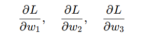
These derivatives guide how each parameter should be updated during training.

3. Second-Order Derivative

The second-order derivative measures how the first derivative changes, indicating the curvature of a function.

📌 Application in AI:

• Helps in advanced optimization techniques like Newton’s method, which improves gradient-based learning by considering the curvature.
• The Hessian matrix, which contains second-order derivatives, is used to analyze how fast or slow the optimization process is converging.

For example, in convex optimization, if the second derivative is positive, the function is convex, meaning we can confidently find a global minimum.

Practical Applications of Derivatives in AI

1. Loss Function Optimization

Every machine learning model aims to minimize the loss function, which measures the difference between predicted and actual values. Derivatives (gradients) guide this process.

• Gradient Descent Algorithm:
  • Uses derivatives to adjust weights and reduce errors.
  • Moves in the direction of the negative gradient to reach the optimal parameter values.

Formula for weight update:

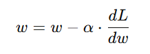
where α is the learning rate, and dL/dw is the gradient of the loss function.

2. Feature Scaling and Importance

Derivatives help in analyzing how sensitive the output of a model is to different input features.

📌 Application in AI:

• Feature selection: If the derivative of the loss function with respect to a feature is close to zero, that feature may not contribute much to the model’s prediction.
• Helps in regularization techniques like L1 and L2 regularization.

3. Neural Network Training & Backpropagation

In deep learning, neural networks adjust weights and biases using backpropagation, which is based on derivatives.

📌 How it works:

1. Forward Pass: The input goes through the network, producing an output.
2. Compute Loss: The difference between predicted and actual values is calculated.
3. Backward Pass (Using the Chain Rule of Derivatives):
   • The loss function’s derivative is computed with respect to each weight.
   • This determines how much each weight contributed to the error.
4. Weights Are Updated Using Gradient Descent.

For a given weight ww, we use the chain rule to compute the gradient:

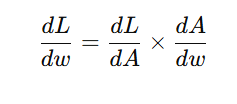
where:

• L is the loss function,
• A is the activation function,
• w is the weight being updated.

Without derivatives, backpropagation would not work, making neural networks unable to learn from data.

Gradients and Gradient Descent: The Backbone of Optimization

In machine learning and deep learning, optimization plays a crucial role in training models effectively. Gradients and gradient descent are fundamental mathematical tools used to minimize errors and improve model performance.

What is a Gradient?

A gradient is a vector containing the partial derivatives of a function with respect to all its input variables. It points in the direction of the steepest ascent of the function.

📌 Why is the gradient important in AI?

• It helps determine how fast and in which direction model parameters should change to minimize the loss function.
• In neural networks, gradients are used to update weights and biases during training.

Mathematically, if we have a function L(w, b) (such as a loss function) dependent on weights w and bias b, its gradient is:

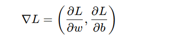
This tells us how much L will change with small changes in w and b.

Gradient Descent Algorithm

Gradient descent is an optimization algorithm that uses gradients to minimize a function (e.g., loss function).

How Gradient Descent Works

1️⃣ Compute the gradient of the loss function with respect to model parameters.
2️⃣ Update parameters by moving in the opposite direction of the gradient (since gradients point to the steepest increase).
3️⃣ Repeat the process iteratively until convergence (i.e., when the loss function reaches its minimum).

📌 Weight update formula:

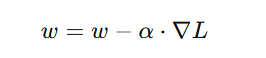
where:

• w = weight parameter
• α = learning rate (controls step size)
• ∇L = gradient of the loss function

This process ensures that the model gradually improves by reducing the error.

Types of Gradient Descent

There are three main types of gradient descent, each with its own trade-offs.

1. Batch Gradient Descent

• Uses the entire dataset to compute the gradient in each iteration.
• Provides stable convergence but can be slow for large datasets.

📌 Best for: Small datasets where computational efficiency is not a major concern.

2. Stochastic Gradient Descent (SGD)

• Updates the model after each sample instead of using the entire dataset.
• Much faster than batch gradient descent but can be noisy, leading to oscillations.

📌 Best for: Large datasets where faster updates are needed, but some noise is acceptable.

3. Mini-Batch Gradient Descent

• A compromise between batch gradient descent and SGD.
• Uses small subsets (mini-batches) of the data for each update.
• Balances efficiency (speed) and stability (less noise).

📌 Best for: Deep learning models, where batch size can be adjusted for optimal training speed and stability.

Practical Applications of Gradients and Gradient Descent

1. Deep Learning Optimization

📌 Neural networks use gradient descent in backpropagation to update weights efficiently.

• The gradient of the loss function determines how weights should be adjusted.
• Backpropagation applies the chain rule of derivatives to propagate errors backward through layers.

2. Hyperparameter Tuning

📌 Learning rates and weight updates depend on gradients.

• If the learning rate is too high, gradient updates overshoot the minimum.
• If the learning rate is too low, learning becomes slow and inefficient.

Using techniques like adaptive gradient methods (Adam, RMSprop, Adagrad), gradient updates can be fine-tuned for better performance.

3. Reinforcement Learning

📌 Gradient-based policy optimization is used in reinforcement learning (RL).

• RL agents learn optimal actions by adjusting their policies based on gradients.
• Techniques like Policy Gradient Methods (e.g., REINFORCE algorithm) rely on gradient computations to improve decision-making in dynamic environments.

Optimization Techniques in AI: From Stochastic Gradient Descent to Adam Optimizer

Optimization is a crucial aspect of AI and machine learning, directly impacting how efficiently models learn and perform. While Gradient Descent is the foundation of optimization, several advanced techniques have been developed to improve speed, stability, and accuracy.

Popular Optimization Methods

1. Momentum-Based Gradient Descent

📌 Concept:

• Traditional gradient descent updates parameters only based on the current gradient.
• Momentum-based gradient descent adds a fraction of the previous update, helping the model move faster in the right direction.

📌 Formula:

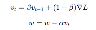
where:

• v_t = velocity (momentum) term
• β = momentum coefficient (typically 0.9)
• α = learning rate
• ∇L = gradient of the loss function

📌 Benefits:
 Reduces oscillations and speeds up convergence.
 Helps in optimizing functions with ravines (steep and narrow valleys).

2. AdaGrad (Adaptive Gradient Algorithm)

📌 Concept:

• Adapts learning rates dynamically for each parameter based on past gradients.
• Parameters with larger gradients get smaller updates, and those with smaller gradients get larger updates.

📌 Formula:

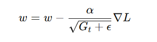
where:

• G_t = sum of squared past gradients
• ε = small smoothing term to prevent division by zero

📌 Benefits:
 Works well for sparse data (e.g., NLP tasks with rare words).
 No need to manually tune the learning rate.

📌 Limitations:
 Learning rate keeps decreasing, which may slow down training in the long run.

3. RMSprop (Root Mean Square Propagation)

📌 Concept:

• Improves upon AdaGrad by considering only recent gradients instead of accumulating all past gradients.
• Helps maintain a consistent learning rate.

📌 Formula:

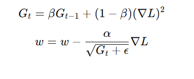
where:

• β = decay factor (typically 0.9)

📌 Benefits:
 Prevents learning rate decay seen in AdaGrad.
 Useful for recurrent neural networks (RNNs) in time-series forecasting.

4. Adam Optimizer (Adaptive Moment Estimation)

📌 Concept:

• Combines Momentum and RMSprop, making it one of the most powerful optimizers.
• Uses two moving averages:
  • First moment (m_t): Momentum-like term for smooth updates.
  • Second moment (v_t): RMSprop-like term to scale learning rates.

📌 Formula:

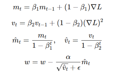
where:

• β₁ = 0.9 (momentum factor)
• β₂ = 0.999 (RMSprop factor)

📌 Benefits:
 Faster convergence and less sensitive to hyperparameter tuning.
 Works well for both small and large datasets.

📌 Limitations:
 Can sometimes overshoot the optimal solution.
 Requires more memory compared to SGD.

Practical Applications of Optimization Techniques

1. Convolutional Neural Networks (CNNs) – Image Processing

• Adam and RMSprop are widely used in training CNNs for tasks like image classification, object detection, and segmentation.
• These optimizers help speed up convergence in deep networks.

2. Natural Language Processing (NLP) – Transformers & LLMs

• AdaGrad and Adam are commonly used in training large-scale transformer models (e.g., BERT, GPT, T5).
• They ensure efficient learning even when dealing with sparse word embeddings.

3. Time-Series Forecasting – Recurrent Neural Networks (RNNs & LSTMs)

• RMSprop and Adam are preferred for training RNNs, LSTMs, and GRUs, which require stable long-term dependencies.
• These optimizers prevent the vanishing/exploding gradient problem.

More Information-Calculus for AI (Derivatives, Gradients, and Optimization)

Next Blog- Probability and Statistics for AI