Feature Engineering and Feature Scaling
Before feeding data into a machine learning or AI model, it's crucial to shape that data into a form the model can learn from effectively. This is where Feature Engineering and Feature Scaling come in — two of the most powerful preprocessing tools in the data science toolbox.
Let’s explore these concepts in detail.
What is Feature Engineering?
Feature Engineering is the process of selecting, transforming, and creating variables (features) that help machine learning models understand the data better. It is more of an art than a science — rooted in domain knowledge, creativity, and logical thinking.
"A model is only as good as the data you feed it."
Poorly designed features will lead to poor performance, no matter how advanced your model is.
Why is Feature Engineering Important?
- Makes patterns in the data easier for the model to detect.
- Reduces noise and redundancy.
- Improves accuracy, recall, precision, and other performance metrics.
- Helps models converge faster during training.
Common Feature Engineering Techniques
Let’s work through the Titanic dataset to apply the most common techniques.
import seaborn as sns
import pandas as pd

# Load Titanic dataset
df = sns.load_dataset('titanic')
df.head()
1. Handling Missing Values
Real-world data is often incomplete. You can either remove rows, fill them with a default value (like mean, median), or use more complex imputation techniques.
# Fill missing 'age' with median
df['age'].fillna(df['age'].median(), inplace=True)

# Drop rows where 'embarked' is missing
df.dropna(subset=['embarked'], inplace=True)
2. Encoding Categorical Variables
ML models work with numbers, not text. So we must convert categories into numerical format.
a. Label Encoding
# Convert 'sex' column into 0 and 1
df['sex'] = df['sex'].map({'male': 0, 'female': 1})
b. One-Hot Encoding
# Convert 'embarked' into multiple binary columns
df = pd.get_dummies(df, columns=['embarked'], drop_first=True)
3. Creating New Features
We can extract new, meaningful information from existing data.
a. Family Size
Combining siblings/spouses (sibsp) and parents/children (parch):
df['family_size'] = df['sibsp'] + df['parch'] + 1
b. Is Child?
Classifying passengers as children based on age:
df['is_child'] = df['age'].apply(lambda x: 1 if x < 18 else 0)
c. Title Extraction (from name)
df['title'] = df['name'].str.extract(' ([A-Za-z]+)\.', expand=False)
Such features often reflect social status and can significantly affect model accuracy.
Absolutely! Let’s expand on Feature Engineering with more advanced techniques and examples, especially in the context of the Titanic dataset and general use-cases in machine learning.
4. Binning (Discretization)
Binning transforms continuous numerical variables into categorical bins. This can help reduce the impact of outliers and reveal non-linear relationships.
a. Age Binning
df['age_bin'] = pd.cut(df['age'], bins=[0, 12, 18, 35, 60, 100],
                       labels=['Child', 'Teen', 'YoungAdult', 'Adult', 'Senior'])
This converts age into distinct life-stage categories.
5. Interaction Features
Sometimes the combination of two or more features captures information that individual features miss.
a. Age * Pclass
df['age_class'] = df['age'] * df['pclass']
This feature could reflect how younger people in higher classes had better survival chances.
6. Frequency Encoding
Instead of one-hot encoding, you can encode categories based on their frequency in the dataset.
a. Encoding Ticket Frequencies
ticket_freq = df['ticket'].value_counts()
df['ticket_freq'] = df['ticket'].map(ticket_freq)
Passengers with the same ticket number might have been traveling together. This feature may capture group survival patterns.
7. Mean/Target Encoding
Assign a value to a category based on the mean of the target variable (like survival rate) within that category.
Use with caution: this technique can cause data leakage if not done properly (should be applied within cross-validation folds).
Example (not applied directly):
df['cabin_survival_mean'] = df.groupby('cabin')['survived'].transform('mean')
8. Text Features (from Names or Tickets)
You’ve extracted titles from names. Let’s go further.
a. Name Length
df['name_length'] = df['name'].apply(len)
Longer or more formal names could indicate social class or family status.
b. Ticket Prefix
df['ticket_prefix'] = df['ticket'].apply(lambda x: ''.join([i for i in x if not i.isdigit()]).strip().replace('.', '').replace('/', ''))
Ticket prefixes can reflect the company or group, offering potential insight into class and survival.
9. Date and Time Features (for time-based datasets)
When working with datetime fields, extract:
- Day of week
- Month
- Hour
- Is weekend?
- Time difference between events (e.g., order → delivery)
Example:
df['order_date'] = pd.to_datetime(df['order_date'])
df['order_dayofweek'] = df['order_date'].dt.dayofweek
df['order_is_weekend'] = df['order_dayofweek'].apply(lambda x: 1 if x >= 5 else 0)
Note: The Titanic dataset doesn’t have datetime fields, but this is common in transactional or time-series data.
10. Log Transformation
To handle skewed features (like fare), apply log transformation:
import numpy as np
df['log_fare'] = np.log1p(df['fare'])  # log1p avoids log(0)
This reduces the impact of extreme outliers and makes distributions more normal.
11. Polynomial Features
Used to capture non-linear relationships between features.
from sklearn.preprocessing import PolynomialFeatures

poly = PolynomialFeatures(degree=2, include_bias=False)
poly_features = poly.fit_transform(df[['age', 'fare']])
12. Scaling and Normalization (Covered Next)
Scaling numerical features ensures that models aren’t biased toward variables with larger magnitude.
Feature Engineering Summary Table
| Technique | Description | Example |
|---|---|---|
| Binning | Convert continuous to categorical | Age → Age Group |
| Interaction Features | Combine features to reveal hidden patterns | Age × Pclass |
| Frequency Encoding | Encode categories based on frequency | Ticket frequency |
| Mean/Target Encoding | Encode category by target mean | Cabin → Mean survival rate |
| Text Features | Use string metrics as features | Name length, ticket prefix |
| Log Transformation | Compress skewed distributions | Fare → log(Fare + 1) |
| Polynomial Features | Create higher-order interactions | Age², Age × Fare |
What is Feature Scaling?
Feature scaling brings all numeric variables into a comparable range so that no single feature dominates the model due to its scale.
Why Scale Features?
Many models are sensitive to the magnitude of features, such as:
- Linear Regression
- Logistic Regression
- K-Nearest Neighbors (KNN)
- Support Vector Machines (SVM)
- Neural Networks
Models like decision trees and random forests do not require scaling.
Popular Feature Scaling Techniques
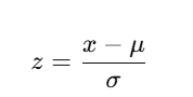
1. Standardization (Z-score Normalization)
Transforms features to have zero mean and unit variance.
Formula:
scaler = StandardScaler()
standardized = scaler.fit_transform(numeric_features)
Use When:
- Data is normally distributed
- Algorithms assume Gaussian distribution (Logistic Regression, SVM, Neural Networks)
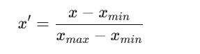
2. Min-Max Scaling
Scales features to a fixed range [0, 1].
Formula:
scaler = MinMaxScaler()
normalized = scaler.fit_transform(numeric_features)
Use When:
- Data does not follow Gaussian distribution
- You want to preserve zero values
- Good for image data (pixel values)
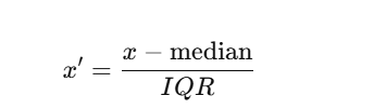
3. Robust Scaling
Scales using median and IQR (interquartile range).
Useful when data contains outliers.
Formula:
scaler = RobustScaler()
robust_scaled = scaler.fit_transform(numeric_features)
Use When:
- Data has outliers (Titanic fare is a great example)
- You want scaling that is not sensitive to outliers
Summary of Key Learnings
| Concept | Goal |
|---|---|
| Feature Engineering | Improve model’s ability to learn patterns from the data |
| Missing Value Treatment | Handle incomplete information |
| Encoding | Convert categorical variables into numeric formats |
| Feature Creation | Extract meaningful insights and representations |
| Feature Scaling | Normalize numerical data to a common scale |
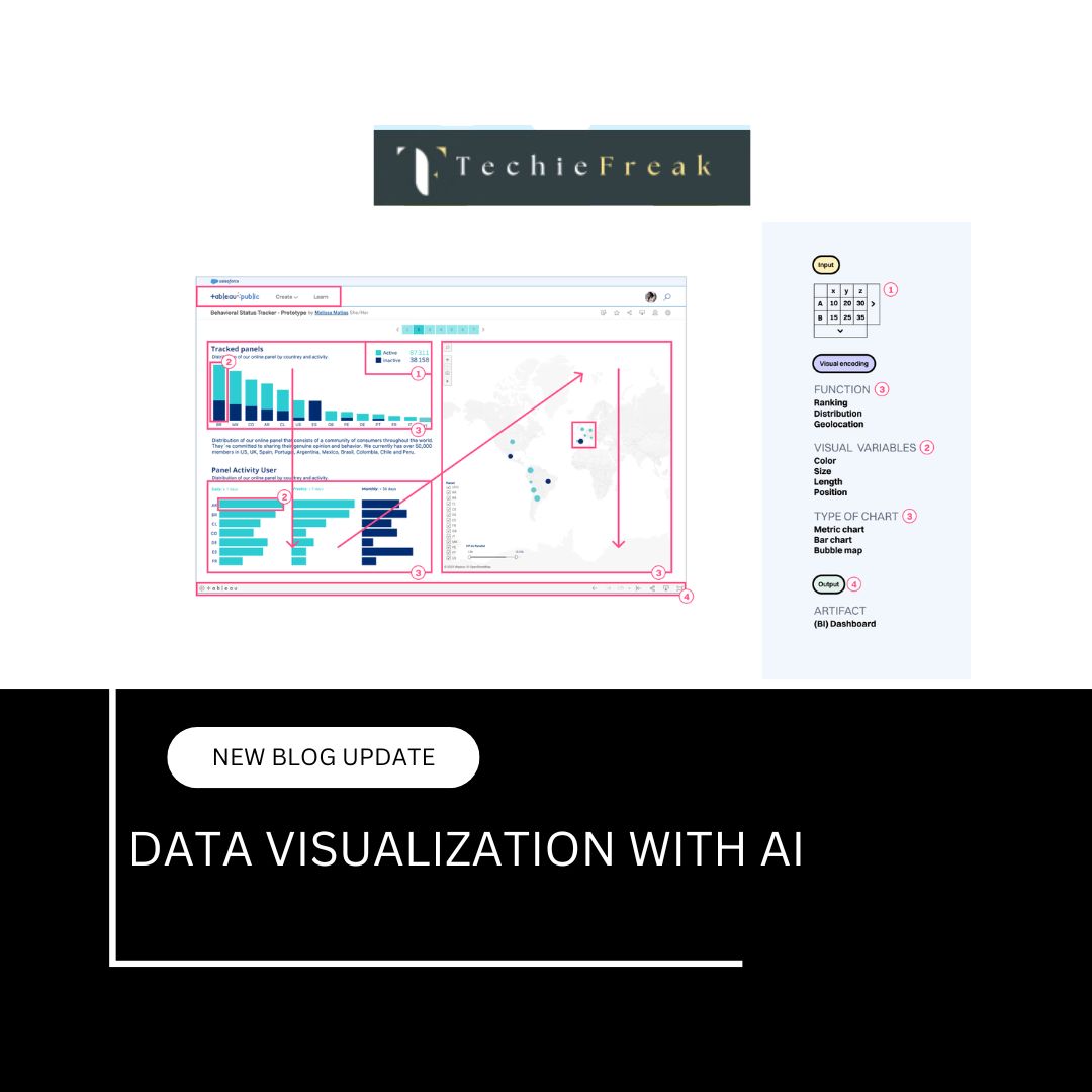
Next Blog- Data Visualization with AI


.jpg)


.jpg)


.png)
.png)
.png)
.png)
.png)
.png)
.png)
.png)
.png)
.png)
.png)
.png)
.png)
.png)
.png)
.png)
.png)
.png)
.png)
.png)
.png)
.png)
.png)
.png)
.png)
.png)
.png)
.png)
.png)
.png)
.png)
.png)
.png)