Python implementation of the Elbow Method 

The Elbow Method is a widely used technique for determining the optimal number of clusters in K-Means Clustering. It involves plotting the Within-Cluster-Sum of Squares (WCSS) for different numbers of clusters and identifying the "elbow point," where the WCSS starts to diminish significantly.

Here is a step-by-step Python implementation of the Elbow Method in K-Means Clustering:

Step 1: Import Required Libraries

We'll start by importing the necessary libraries: numpy, pandas, scikit-learn for model building, and matplotlib for visualization.

import numpy as np
import matplotlib.pyplot as plt
from sklearn.cluster import KMeans
from sklearn.datasets import make_blobs

Step 2: Generate or Load Data

Create synthetic data using make_blobs or read the data from some of the open repositories like Kaggle dataset, UCI Machine Learning Repository etc and explore the data to understand the features and its importance.

# Generate synthetic data for clustering
X, y = make_blobs(n_samples=300, centers=4, cluster_std=1.0, random_state=42)

# Display the first few rows of data
print("Features: \n", X[:5])
print("Target: \n", y[:5])

OUTPUT:
Input Features: 
 [[ -9.29768866   6.47367855]
 [ -9.69874112   6.93896737]
 [ -1.68665271   7.79344248]
 [ -7.09730839  -5.78133274]
 [-10.87645229   6.3154366 ]]
 
 

Target: 
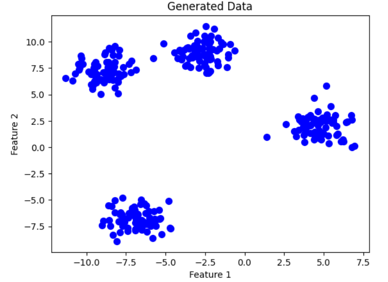
 [3 3 0 2 3]

Step 3: Visualize the Data (Optional)

Plot the dataset to understand its structure.

plt.scatter(X[:, 0], X[:, 1], s=50, c='blue')
plt.title("Generated Data")
plt.xlabel("Feature 1")
plt.ylabel("Feature 2")
plt.show()

Step 4: Calculate WCSS for Different Number of Clusters

Loop through a range of cluster values ranges from 1-11 here in this example. you can choose the different range and calculate the WCSS for each.

wcss = []  # To store Within-Cluster Sum of Squares

# Try K values from 1 to 10
for i in range(1, 11):
    kmeans = KMeans(n_clusters=i, init='k-means++', random_state=42)
    kmeans.fit(X)
    wcss.append(kmeans.inertia_)  # Inertia is the WCSS for the KMeans model

print(wcss)

OUTPUT:
[19953.769148278025, 9416.214004352278, 2110.4125218953286, 564.9141808210254, 513.0329042790801, 462.0960007878173, 411.3489318727926, 365.355599299591, 332.03645710154746, 291.5608624106774]

Step 5: Plot the Elbow Curve

Plot the WCSS values with respect to no of clusters to visualize the elbow point.

plt.figure(figsize=(8, 5))
plt.plot(range(1, 11), wcss, marker='o', linestyle='--', color='b')
plt.title('Elbow Method for Optimal K')
plt.xlabel('Number of Clusters (K)')
plt.ylabel('WCSS')
plt.xticks(range(1, 11))
plt.show()

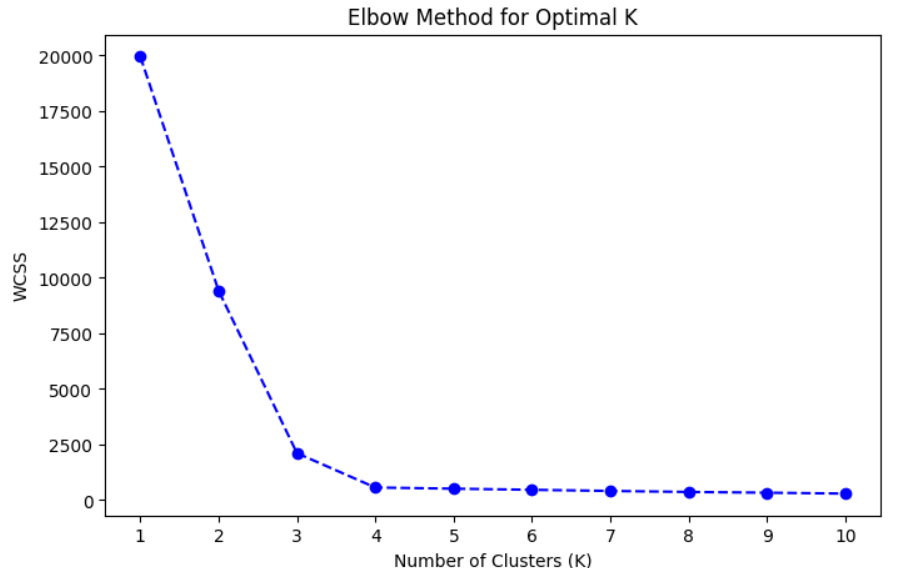
Step 6: Identify the Elbow Point

Manually inspect the plot to identify the "elbow" point where the WCSS starts to drop less significantly. If we see the above graph, it  clearly shows that after the k=4, the value of wcss is not decreasing that much o we can say that k=4 is optimal no of clusters.

Alternatively, you can use methods of the KneeLocator library of the package kneed, which can be used to detect the knee point or elbow point  by implementing the Kneedle algorithm. We will create a separate blog for this where we will discuss this in detail.

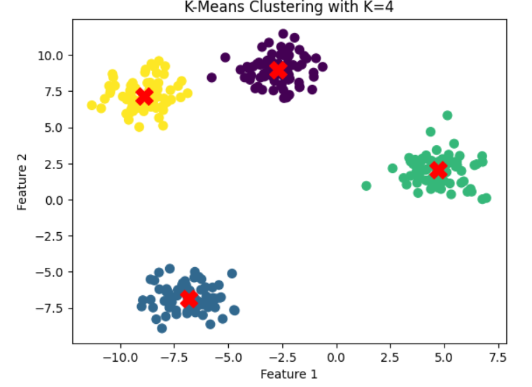
Step 7: Apply K-Means with Optimal K

Use the identified optimal number of clusters for the final K-Means clustering.

# Assume the elbow point is at K=4
optimal_k = 4
kmeans = KMeans(n_clusters=optimal_k, init='k-means++', random_state=42)
y_kmeans = kmeans.fit_predict(X)

# Visualize the clusters
plt.scatter(X[:, 0], X[:, 1], c=y_kmeans, s=50, cmap='viridis')
centers = kmeans.cluster_centers_  # Cluster centers
plt.scatter(centers[:, 0], centers[:, 1], c='red', s=200, marker='X')  # Highlight cluster centers
plt.title(f"K-Means Clustering with K={optimal_k}")
plt.xlabel("Feature 1")
plt.ylabel("Feature 2")
plt.show()

Summary of Steps:

1. Import necessary libraries.
2. Generate or load the dataset.
3. Visualize the data (optional).
4. Compute WCSS for different K values.
5. Plot the Elbow Curve to identify the optimal K.
6. Apply K-Means clustering using the optimal number of clusters.
7. Visualize the final clusters.

Next Blog- Python implementation of the Silhouette Method in K-Means Clustering