Introduction to Linear Discriminant Analysis (LDA)

Linear Discriminant Analysis is used when the dependent variable is categorical, making it a classification algorithm. It assumes that different classes generate data based on Gaussian distributions and tries to maximize the separability between these classes by minimizing the intra-class variance and maximizing the inter-class variance.

LDA is particularly effective when dealing with linearly separable classes, although it can still perform reasonably well for slightly overlapping classes.

Goals of LDA

LDA aims to:

1. Maximize Class Separation: Project the data onto a lower-dimensional space where the separation between classes is maximized.
2. Reduce Dimensionality: Find a new feature space (lower-dimensional) while retaining as much class-discriminatory information as possible.

Theory Behind LDA

1. Assumptions of LDA

Linear Discriminant Analysis (LDA) is a supervised machine learning algorithm used for classification. It makes several key assumptions about the data, which helps simplify the computation and improve performance when these assumptions hold true. Here's a breakdown of each assumption:

1. Data for Each Class is Drawn from a Gaussian (Normal) Distribution:
   • Explanation: LDA assumes that the data points for each class follow a Gaussian (normal) distribution. This means that within each class, the features (variables) should have a bell-shaped distribution where the mean and standard deviation define the center and spread of the data.
   • Implication: This assumption implies that the data from each class should be well-approximated by a normal distribution, with a peak around the mean and symmetrically distributed around it. This is important because LDA uses the probability distribution of each class to classify new data points.
   • Real-World Example: If you're classifying two species of flowers, LDA assumes that the measurements for each species (such as petal length or width) follow a normal distribution for each feature.
2. Each Class Has the Same Covariance Matrix (Homoscedasticity):
   • Explanation: LDA assumes that the covariance matrix (which represents how features vary together) is the same for all classes. This means the spread and correlation between features are assumed to be identical across different classes. The idea is that each class has the same "shape" or "scatter" in the feature space.
   • Implication: In practice, this assumption means that the variance (spread) and covariance (relationships between features) of the data for each class should be equal. If this assumption is violated, LDA might perform poorly because the decision boundaries between classes might not be well defined.
   • Real-World Example: In a dataset with two classes of customers, one for high-income individuals and another for low-income individuals, LDA assumes that the variability in features like age or education level is similar for both classes.
3. Classes Are Linearly Separable in the Transformed Space:
   • Explanation: LDA assumes that after projecting the data onto a lower-dimensional space (often through a linear combination of the features), the classes become separable by a linear boundary (a straight line in 2D, a plane in 3D, or a hyperplane in higher dimensions).
   • Implication: LDA tries to find the linear combination of features that best separates the classes. The assumption here is that even if the classes overlap in the original feature space, they can be separated using a linear decision boundary once transformed. This linear separation simplifies the classification process.
   • Real-World Example: In a dataset with two classes, such as classifying emails as "spam" or "not spam," LDA assumes that the emails can be separated into two groups by a straight line (or a hyperplane in a higher-dimensional space) based on certain features like word frequency.

Why Are These Assumptions Important?

• Gaussian Distribution: This allows LDA to model the data from each class using probability theory and calculate the likelihood of a data point belonging to each class.
• Equal Covariance Matrix: This assumption simplifies the model by assuming that the "spread" of data is the same across classes, allowing for a simpler calculation of the decision boundary.
• Linearly Separable Classes: This assumption enables the use of linear decision boundaries, which are computationally simpler and more efficient, while also reducing the complexity of the model.

If these assumptions hold true, LDA can perform well and provide good classification results. However, if the assumptions are violated (e.g., if classes have different variances or the data is not normally distributed), the performance of LDA may degrade, and alternative algorithms like Quadratic Discriminant Analysis (QDA) or non-linear classifiers may be more appropriate.

2. Mathematical Representation

a. Dataset Representation

Let:

• X={x1,x2,…,xn}  be the dataset with n samples.
• Each sample xi ∈Rd is a vector in d-dimensional space.
• k is the number of classes, and each class is denoted by C1,C2,…,Ck.
• ni is the number of samples in class Ci​.

b. Mean Vectors

In LDA, the mean vectors are crucial for computing the decision boundaries that separate different classes. Mean vectors are used to represent the "average" data point of a particular class and the entire dataset.

1. Class Mean (μi​): The class mean vector represents the average of all the feature values for each individual class. The mean vector for each class Ci​ is calculated as:

   

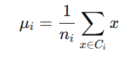
Where:

• x∈Ci indicates that x is a sample belonging to class Ci​.
• ni​ is the number of samples in class Ci​.
• μi​ is the mean vector for class Ci, which is a vector of the mean values for each feature in class Ci​.
   
• Purpose: The class mean vector gives us the central point (average) for each class in the feature space. By comparing these class mean vectors, we can understand how different the classes are in terms of their feature distributions.
• Example: Suppose you have a dataset of two features, "Height" and "Weight", and you are classifying data into two classes: "Male" and "Female". The class mean vector for "Male" would be the average height and weight of all male samples in the dataset, while the class mean vector for "Female" would be the average height and weight of all female samples.

1. Overall Mean (μ\muμ): The overall mean vector represents the mean of the entire dataset, i.e., the average of all the feature values across all classes combined. The overall mean of the entire dataset is calculated as:

   

   

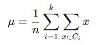
Where:

• x∈X represents all samples in the dataset.
• N is the total number of samples in the dataset (across all classes).
• μ is the overall mean vector, which is a vector of the mean values of each feature across the entire dataset.
   
• Purpose: The overall mean vector serves as a reference point for all classes. It is used in LDA to measure how much each class differs from the entire dataset in terms of the average feature values. This is important when calculating the between-class scatter matrix.
• Example: Using the same "Male" and "Female" classes with features "Height" and "Weight", the overall mean vector would be the average height and weight across all males and females combined.

c. Scatter Matrices

In LDA, scatter matrices are used to measure and quantify the variance or spread of data within and between classes. These matrices help LDA identify which directions in the feature space best separate different classes, aiding in dimensionality reduction and classification.

Scatter matrices are crucial for understanding how data points are distributed within each class (within-class scatter) and how distinct the classes are from each other (between-class scatter).

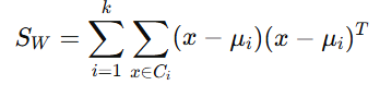
1) Within-Class Scatter Matrix (SW​)

The within-class scatter matrix quantifies how much the data points within each class deviate from their respective class means. It is used to measure the spread of data within each class. The smaller the within-class scatter matrix, the more compact the data is within each class, which is desirable for classification. The within-class scatter matrix quantifies the spread of data points within each class:

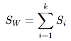
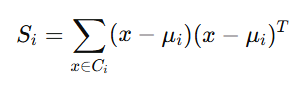
where Si is the scatter matrix for class Ci, defined as:

Thus, SW​ becomes:

2)  Between-Class Scatter Matrix (SB​)

The between-class scatter matrix quantifies the spread between the mean vectors of the different classes. It measures how distinct each class is from the overall mean of the entire dataset. The larger the between-class scatter matrix, the more separated the classes are from each other, which is desirable for classification. The between-class scatter matrix quantifies the spread between the mean vectors of the classes:

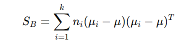
Here:

• (μi−μ)  is the distance of class iii’s mean from the overall mean.
• ni weights the contribution of each class by its sample size.

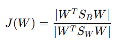
d. The Optimization Problem

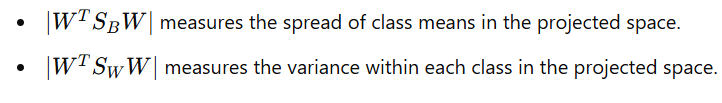
In Linear Discriminant Analysis (LDA), the goal is to find a projection matrix W that transforms the data into a new subspace where the classes are as separable as possible. The separability is quantified by comparing the between-class variance and within-class variance. LDA seeks to find a projection matrix W such that the projected data maximizes the separability between classes. This is achieved by maximizing the ratio of:

1. Between-class variance (numerator) to
2. Within-class variance (denominator).

Fisher Criterion

The Fisher Criterion provides the optimization objective for LDA. It aims to maximize the ratio of between-class variance (how well-separated the class means are) to within-class variance (how compact the classes are).

The Fisher criterion can be expressed as: 

where:

e.  Solving the Eigenvalue Problem

To maximize J(W) , the problem reduces to solving the generalized eigenvalue problem:

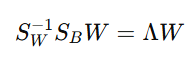
where:

• Λ is a diagonal matrix containing the eigenvalues.
• W is the matrix of eigenvectors.

1) Eigenvectors

• The eigenvectors corresponding to the largest eigenvalues form the projection matrix W.
• These eigenvectors define the new axes onto which the data is projected.

2) Dimensionality of W

• If there are k classes, W will have at most k−1 eigenvectors, since the rank of SB​ is at most k−1

f.  Data Projection

In Linear Discriminant Analysis (LDA), after finding the optimal projection matrix W, the next step is to project the original high-dimensional data onto a lower-dimensional space. This helps reduce the dimensionality of the data while retaining the most discriminative features for class separability. The data is projected onto the lower-dimensional space using the projection matrix W:

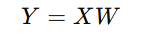
where:

• X is the original dataset of size n×d
• W is the projection matrix of size d×(k−1)
• Y is the transformed dataset of size n×(k−1)

g. Classification in Transformed Space

After projection, classification is typically performed in the lower-dimensional space Y. This is often done by:

1. Assigning to the Nearest Mean: For a new data point, calculate its distance to the mean of each class in the transformed space and assign it to the nearest class.
2. Using other classifiers such as logistic regression or k-NN.

Strengths and Applications of LDA

Strengths

1. Efficient Dimensionality Reduction: Reduces high-dimensional data to a smaller subspace while preserving class separability.
2. Simple Implementation: The linear nature of the algorithm makes it computationally efficient.
3. Feature Interpretability: The resulting components (linear discriminants) provide interpretable features for classification.

Applications

1. Face Recognition: Used to reduce dimensionality in image data (e.g., Eigenfaces).
2. Medical Diagnostics: Identifying diseases based on features like symptoms or biomarkers.
3. Marketing Segmentation: Classifying customer groups based on behavioral data.

Limitations of LDA

1. Linear Assumption: LDA struggles with non-linear class boundaries.
2. Gaussian Assumption: The performance degrades if the data distribution significantly deviates from normality.
3. Covariance Assumption: Homoscedasticity may not always hold in real-world datasets.

Key Takeaways:

• Linear Discriminant Analysis (LDA) is a classification algorithm used for categorical dependent variables.
• Goals of LDA:
  • Maximize class separation.
  • Reduce dimensionality while retaining class-discriminative information.
• Assumptions:
  • Gaussian Distribution: Data for each class follows a normal distribution.
  • Equal Covariance Matrix (Homoscedasticity): All classes have the same covariance matrix.
  • Linearly Separable: Classes are separable in a transformed (lower-dimensional) space.
• Mathematical Representation:
  • Mean Vectors: Represent the average feature values for each class and the overall dataset.
  • Scatter Matrices:
    • Within-Class Scatter Matrix: Measures data spread within each class.
    • Between-Class Scatter Matrix: Measures how distinct the classes are from each other.
• Optimization:
  • LDA maximizes the Fisher Criterion (ratio of between-class variance to within-class variance) to find the optimal projection matrix WW.
• Data Projection:
  • Project the original data onto a lower-dimensional space to achieve class separability.
• Classification:
  • Classification is done in the transformed space by assigning new points to the nearest class mean or using other classifiers.
• Strengths:
  • Efficient dimensionality reduction.
  • Simple to implement and computationally efficient.
  • Provides interpretable features for classification.
• Applications:
  • Face recognition, medical diagnostics, and marketing segmentation.
• Limitations:
  • Struggles with non-linear class boundaries.
  • Performance degrades if the Gaussian or covariance assumptions are violated.

Next Blog- Python implementation of Linear Discriminant Analysis (LDA)