.png)
Non-Negative Matrix Factorization (NMF)
Non-Negative Matrix Factorization (NMF) is a machine learning and linear algebra technique for dimensionality reduction and data representation. It decomposes a non-negative matrix V into two lower-dimensional non-negative matrices, W and H, where:
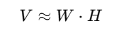
This decomposition provides a way to approximate V while reducing its dimensions, where:
- V: Original matrix of size m×n(e.g., a document-term matrix in NLP, image pixel intensity matrix, etc.).
- W: Basis matrix of size m×k(non-negative matrix capturing latent features).
- H: Coefficient matrix of size k×n (non-negative matrix representing the weight of these latent features for each sample).
The non-negativity constraint ensures all elements of V, W, and H are greater than or equal to zero, making the results interpretable. This is especially useful for applications like text, image, and bioinformatics, where negative values are not meaningful.
Key Objectives of NMF
- Dimensionality Reduction: NMF reduces high-dimensional data into smaller latent dimensions, retaining meaningful patterns.
- Feature Extraction: It identifies parts-based representations (e.g., components of images or topics in text).
- Data Interpretation: Non-negativity constraints allow for intuitive interpretation of results.
Applications of NMF
- Natural Language Processing (NLP):
- Topic modeling: Decomposing a document-term matrix to extract topics and their weights.
- Image Processing:
- Separating images into parts (e.g., facial components like eyes, nose, and mouth).
- Audio Source Separation:
- Decomposing audio signals to isolate different instruments or vocals.
- Recommender Systems:
- Reducing sparse user-item matrices to identify latent preferences.
- Bioinformatics:
- Gene expression analysis to identify gene clusters or pathways.
Mathematical Representation
NMF seeks to minimize the reconstruction error between VVV and W⋅HW \cdot HW⋅H. Two commonly used objective functions are:
1. Frobenius Norm
What is the Frobenius Norm?
The Frobenius norm of a matrix is a way to measure the difference (error) between two matrices. It is calculated as the square root of the sum of the squares of all elements in the matrix. For a matrix A, the Frobenius norm is defined as:
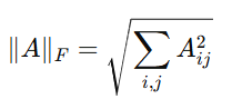
It is commonly used in Non-negative Matrix Factorization (NMF) and error minimization problems.
What are V, W, and H?
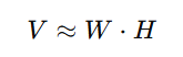
- In Non-negative Matrix Factorization (NMF), we decompose a large matrix V into two smaller matrices W and H:
Where:
- V (Original Data Matrix): This is the matrix we want to factorize. It usually represents a dataset where each row is a data point and each column is a feature.
- W (Basis Matrix): Contains the "building blocks" or "patterns" that are combined to approximate V.
- H (Coefficient Matrix): This represents how strongly each pattern in W contributes to reconstructing V.
Why Minimize the Frobenius Norm?
The goal of NMF is to find W and H such that the error (difference between V and W⋅H) is minimized. This is done by minimizing the Frobenius norm of the error matrix:
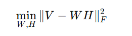
This ensures that the factorization is as close as possible to the original matrix.
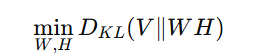
2. Kullback-Leibler (KL) Divergence
KL divergence is another way to measure the difference between the original matrix V and its factorized approximation W⋅H. Instead of using the Frobenius norm (sum of squared differences), it measures how much information is lost when approximating V with W⋅H.
An alternative formulation minimizes the divergence between the original matrix V and its approximation W⋅H:
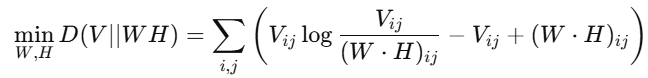
Why Use KL Divergence in NMF?
Instead of minimizing the squared difference like in the Frobenius norm, minimizing KL divergence focuses on preserving the distribution of the original data. This is useful in applications like text processing and image processing, where data often follows a probabilistic distribution.
The optimization problem in KL-based NMF is:
This means we are adjusting W and H such that the approximation WH s as statistically similar to V as possible.
Constraints and Properties
Non-Negativity:
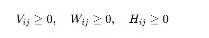
- This ensures that all values in V,W,H remain non-negative.
- Important in applications like topic modeling, image decomposition, and bioinformatics, where negative values don’t make sense (e.g., frequency counts in text or pixel intensities in images).
- Dimensionality:
- The rank of the matrices W and H (i.e., k) is typically much smaller than the original matrix V, which achieves dimensionality reduction.
When to Use KL Divergence vs. Frobenius Norm?
| Method | Best Used For | Characteristics |
|---|---|---|
| Frobenius Norm | General-purpose NMF, noise reduction | Minimizes squared error, good for numerical accuracy |
| KL Divergence | Probability-based applications (text, images) | Focuses on preserving data distribution, better for sparse data |
Optimization Techniques
- Since the objective function is not convex in W and H simultaneously, NMF optimization is done iteratively. Common techniques include
1. Multiplicative Update Rules
This is the most widely used method for NMF. It ensures non-negativity by updating W and H iteratively using a multiplicative approach.
Update Formulas:
The iterative update rules for W and H are:
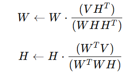
How It Works:
- Each element of W and H is updated proportionally using the corresponding elements in V.
- The updates ensure that negative values never appear, maintaining the non-negativity constraint.
- The process is repeated until convergence, i.e., when the error ∥V−WH∥ stops decreasing significantly.
- These updates are repeated until convergence, i.e., when the reconstruction error stops decreasing significantly.
2. Alternating Least Squares (ALS)
In ALS, instead of updating both W and H simultaneously, we update one matrix at a time while keeping the other fixed.
Steps in ALS:
Fix W and solve for H using least squares optimization:
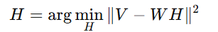
Fix H and solve for W:
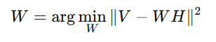
- Repeat until convergence (i.e., until ∥V−WH∥ stops changing significantly).
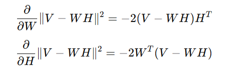
3. Gradient Descent
This method minimizes the objective function by computing gradients and updating W and H in the opposite direction of the gradient.
Update Formulas:
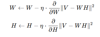
Where η is the learning rate.
Gradient Calculation:
How It Works:
- The gradients tell us how to adjust W and H to reduce the reconstruction error.
- We update W and H iteratively using the learning rate η to control step size.
- If an update causes negative values, we either clip them to zero or add a penalty term.
Advantages of NMF
- Interpretability:
- The non-negativity constraints result in parts-based, intuitive representations (e.g., topics in text or parts of an image).
- Efficient Dimensionality Reduction:
- Suitable for sparse and high-dimensional data.
- Scalability:
- Can handle large datasets effectively.
Limitations of NMF
- Non-Convex Optimization:
- The optimization problem is not convex in both W and H, leading to multiple local minima.
- Dependency on Initialization:
- Results depend heavily on the initial values of W and H, requiring careful tuning.
- Sensitivity to Noise:
- NMF can be sensitive to noise in the data, which may affect interpretability.
Key Takeaways-
- Dimensionality Reduction: NMF reduces high-dimensional data into smaller latent matrices while retaining important patterns.
- Feature Extraction: It helps identify meaningful components, like topics in text or parts of images.
- Non-Negativity Constraint: Ensures all values in the matrices (V, W, H) are non-negative, making the results interpretable.
- Applications: NMF is used in NLP (topic modeling), image processing, audio source separation, and bioinformatics.
- Objective Functions: NMF can use Frobenius Norm (for general-purpose, noise reduction) or KL Divergence (for probabilistic, sparse data applications).
- Optimization Techniques: Common methods include Multiplicative Update Rules, Alternating Least Squares (ALS), and Gradient Descent.
- Advantages: Provides intuitive, parts-based representations and is scalable for large datasets.
- Limitations: Non-convex optimization, sensitivity to initialization and noise.
Next Blog- Python Implementation of Non-Negative Matrix Factorization (NMF)

.png)
.png)
.png)
.png)
.png)
.png)
.png)
.png)
.png)
.png)
.png)
.png)
.png)
.png)
.png)
.png)
.png)
.png)
.png)
.png)
.png)
.png)
.png)