Introduction: 

Locally Linear Embedding (LLE) is a popular non-linear dimensionality reduction technique that maps high-dimensional data to a lower-dimensional space while preserving the local relationships between neighboring data points. It is particularly useful for datasets with non-linear structures, such as those lying on a manifold.

Key Concepts Behind LLE

1. Dimensionality Reduction:

• In many machine learning tasks, data lies in a high-dimensional space but is often embedded in a lower-dimensional manifold. For example, a 3D surface may be embedded in a 2D plane.
• The goal of LLE is to find this low-dimensional representation while preserving the local geometric relationships of the data.

2. Local Linear Relationships:

• LLE assumes that each data point and its neighbors lie on or near a locally linear patch of the manifold.
• The high-dimensional relationships among neighboring points are preserved in the low-dimensional embedding.

How LLE Works

LLE involves three main steps:

Step 1: Find the Nearest Neighbors

For each data point xi in the dataset:

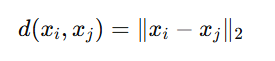
• Compute the k-nearest neighbors (using distance metrics like Euclidean distance).
• These neighbors define the "local neighborhood" of xi

Step 2: Compute Reconstruction Weights

• The algorithm assumes that each point can be approximately reconstructed as a weighted linear combination of its neighbors.

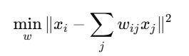
• For a point xi, we solve: 

  

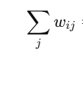
  Subject to:

  

• where:
  • wij are the reconstruction weights for the neighbors of xi
  • The weights are computed such that they minimize the reconstruction error,
  • The constraint ensures that weights are normalized.

Step 3: Compute Low-Dimensional Embedding

• In the low-dimensional space, we aim to preserve the same reconstruction weights computed in the high-dimensional space.
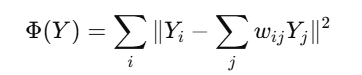
• Solve the eigenvalue problem to find the low-dimensional representation Y that minimizes the cost:

• Here:
  • Yi​ represents the low-dimensional embedding of xi
  • wij​ are the reconstruction weights obtained in Step 2.
• The solution is found by computing the eigenvectors of a matrix derived from the reconstruction weights.

Mathematical Representation of Locally Linear Embedding (LLE)

Locally Linear Embedding (LLE) maps high-dimensional data to a lower-dimensional space by preserving the local relationships among neighboring points. Below is the detailed step-by-step mathematical representation of the LLE algorithm:

1. Input

• X={x1​,x2​,…,xn​}, a set of n data points in RD (high-dimensional space).
• Output: Y={y1,y2,…,yn}, the corresponding data points in Rd (low-dimensional space), where d≪Dd.

 Step 1: Identify the Nearest Neighbors

For each point xi∈RD

• Compute the k-nearest neighbors of xi based on the Euclidean distance:

• Let Ni​ denote the set of indices corresponding to the k-nearest neighbors of xi.

Step 2: Compute Reconstruction Weights

Each data point xi is approximated as a weighted linear combination of its neighbors:

Objective Function for Weights:

The Objective Function for Weights in LLE is the function that needs to be minimized in order to find the optimal set of weights. The goal is to reconstruct each data point as a weighted sum of its nearest neighbors while minimizing the reconstruction error.

• Reconstruction Error: The error is the difference between the original data point xi and the weighted sum of its neighbors. Minimizing this error ensures that the relationship between data points in the high-dimensional space is preserved.
• Normalization Constraint: The weights are normalized to ensure that their sum equals 1. This prevents the model from giving excessive importance to any single neighbor.

Thus, the objective function for weights can be written as:

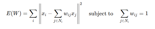
By solving this minimization problem, we get the weights matrix W, which captures the local linear relationships between each data point and its neighbors.

Solution for Weights:

The Solution for Weights refers to finding the set of weights that best reconstruct each data point from its neighbors in the high-dimensional space. The reconstruction weights wij​ are found by solving a minimization problem that reduces the error between the original point and its linear combination of neighbors. This is achieved by solving the following:

• For each data point xi, we approximate it as a weighted sum of its nearest neighbors:

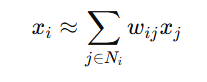
where Ni is the set of nearest neighbors of xi, and wij are the reconstruction weights.

• The objective function to minimize is the reconstruction error, which is the difference between the point xix_ixi​ and the weighted sum of its neighbors:

  

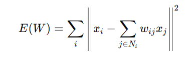
  The minimization ensures that the data point xix_ixi​ is well approximated by its neighbors in the high-dimensional space.

• The weights wij​ must also satisfy a normalization constraint:

  

This ensures that the weights are balanced and prevent any data point from being "over-emphasized."

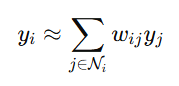
Step 3: Compute the Low-Dimensional Embedding

The goal is to find the low-dimensional representation Y={y1,y2,…,yn} such that the same reconstruction weights WWW are preserved in the low-dimensional space:

Objective Function for Embedding:

Minimize the cost function:

Matrix Formulation:

1. Construct a sparse weight matrix W such that:

   

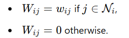
2. Define the matrix M:

   

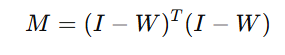
   where I is the identity matrix.

3. Solve the eigenvalue problem:

   

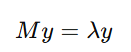
   The d+1 smallest eigenvalues (excluding the smallest eigenvalue, which is zero) correspond to the low-dimensional embedding Y.

Output

• The embedding Y is formed from the eigenvectors corresponding to the d+1smallest eigenvalues of M, excluding the eigenvector associated with the smallest eigenvalue (which corresponds to the centroid of the data).

Key Matrices in LLE

1. Weight Matrix W: Captures the local linear reconstruction of data points in high dimensions.
2. Embedding Cost Matrix M: Encodes the preservation of local relationships during dimensionality reduction.

Advantages of LLE

1. Non-Linearity: Unlike PCA, LLE captures non-linear structures in the data.
2. Manifold Learning: Effectively maps data lying on non-linear manifolds to a low-dimensional space.
3. No Local Minima: The eigenvector computation ensures a global optimum solution.

Limitations of LLE

1. Computational Cost: The eigenvalue decomposition can be computationally expensive for large datasets.
2. Choice of Parameters:
   • The number of neighbors k significantly affects the results.
   • Too few neighbors may fail to capture the manifold structure, while too many may dilute the locality.
3. Sensitivity to Noise: LLE can be sensitive to noise in the data, which can affect the neighborhood relationships.

Applications of LLE

1. Visualization: Reducing high-dimensional data for 2D or 3D visualization.
2. Preprocessing: Dimensionality reduction before clustering, classification, or regression tasks.
3. Image Processing: Finding low-dimensional representations of images or video sequences.
4. Bioinformatics: Analyzing high-dimensional genomic or proteomic data.

Key Takeaways

1. LLE is a Non-Linear Dimensionality Reduction Method: It reduces high-dimensional data to a lower-dimensional space while preserving local relationships.
2. Step-by-Step Process:
   • Step 1: Find the nearest neighbors for each data point.
   • Step 2: Compute reconstruction weights to represent each data point as a linear combination of its neighbors.
   • Step 3: Solve an eigenvalue problem to find the low-dimensional embedding that preserves these local relationships.
3. Mathematical Formulation:
   • We minimize reconstruction error in high dimensions.
   • Reconstruction weights are subject to a normalization constraint.
   • The final low-dimensional embedding is obtained through eigenvalue decomposition.
4. Advantages of LLE:
   • Effectively captures non-linear relationships in data.
   • Suitable for manifold learning and data with non-linear structures.
   • No local minima in the eigenvector calculation, ensuring a global optimum.
5. Limitations of LLE:
   • Computationally expensive for large datasets due to eigenvalue decomposition.
   • Sensitive to the number of neighbors (k), affecting the structure captured.
   • Vulnerable to noise, which may affect the results.
6. Applications of LLE:
   • Data visualization in 2D or 3D.
   • Preprocessing for clustering, classification, or regression tasks.
   • Image processing, bioinformatics, and other high-dimensional data analysis.

Next Blog- Step-wise Python Implementation of Locally Linear Embedding (LLE)