Python implementation of Divisive Hierarchical Clustering
 

Divisive Hierarchical Clustering (DIANA: DIvisive ANAlysis) is a top-down clustering method. It starts with all data points in a single cluster and recursively splits them into smaller clusters until each point is in its cluster or the stopping criterion is met.

Here's a step-by-step Python implementation of Divisive Hierarchical Clustering:

Step 1: Import Required Libraries

We'll start by importing the necessary libraries: numpy, pandas, scikit-learn for model building, and matplotlib for visualization.

import numpy as np
import matplotlib.pyplot as plt
from scipy.spatial.distance import pdist, squareform
from sklearn.datasets import make_blobs

Step 2: Generate or Load Data

In this step we will read the data from some of the open repositories like Kaggle dataset, UCI Machine Learning Repository etc and explore the data to understand the features and its importance.

Here, we'll generate some random data or use an example dataset to demonstrate the clustering.

# Generate synthetic data
X, y = make_blobs(n_samples=10, centers=2, cluster_std=1.5, random_state=42)
print("Input Features : ")
print(X[:5])

print("Target:  ")  
print(y[:5])

OUTPUT:
Input Features : 
[[ 2.05250209  1.12973839]
 [-3.20432416  8.3156915 ]
 [-0.1403784  10.16543822]
 [ 3.12063216  2.44454068]
 [-2.86042769  8.66308069]]
Target:  
[1 0 0 1 0]

Step 3: Compute Pairwise Distance Matrix

Calculate the distance matrix using a distance metric (e.g., Euclidean distance).

# Compute the pairwise distance matrix
distance_matrix = squareform(pdist(X, metric='euclidean'))
print("Pairwise Distance Matrix:\n", distance_matrix)

OUTPUT:

Pairwise Distance Matrix:
 [[ 0.          8.90349057  9.29798883  1.69399141  8.99378259  1.76837398
   2.98371876  6.54033961 10.16817447  4.81239533]
 [ 8.90349057  0.          3.57901196  8.62991798  0.48881903 10.65864088
  11.62046727  2.41540213  1.51246198 12.06207255]
 [ 9.29798883  3.57901196  0.          8.38131545  3.10736967 10.86256263
  11.42479062  4.49361341  3.09148795 11.0217737 ]
 [ 1.69399141  8.62991798  8.38131545  0.          8.62805405  2.59459375
   3.070893    6.43652062  9.72817634  3.80494391]
 [ 8.99378259  0.48881903  3.10736967  8.62805405  0.         10.73618578
  11.64906955  2.61800853  1.21734423 11.97777943]
 [ 1.76837398 10.65864088 10.86256263  2.59459375 10.73618578  0.
   1.46344748  8.30545274 11.89980251  3.9805631 ]
 [ 2.98371876 11.62046727 11.42479062  3.070893   11.64906955  1.46344748
   0.          9.33978097 12.77172608  2.76271932]
 [ 6.54033961  2.41540213  4.49361341  6.43652062  2.61800853  8.30545274
   9.33978097  0.          3.83521977 10.0529593 ]
 [10.16817447  1.51246198  3.09148795  9.72817634  1.21734423 11.89980251
  12.77172608  3.83521977  0.         12.96816593]
 [ 4.81239533 12.06207255 11.0217737   3.80494391 11.97777943  3.9805631
   2.76271932 10.0529593  12.96816593  0.        ]]

Step 4: Initialize a Single Cluster

In this we start with all points in single cluster.

# Initially, all data points belong to a single cluster
clusters = [list(range(len(X)))]  # A list of clusters, each cluster is a list of indices

Step 5: Define a Split Function

Create a function to split a cluster into two clusters based on maximum dissimilarity.

def split_cluster(distance_matrix, cluster):
    # Find the pair of points with the largest distance
    sub_matrix = distance_matrix[np.ix_(cluster, cluster)]  # Sub-matrix for the current cluster
    farthest_points = np.unravel_index(np.argmax(sub_matrix), sub_matrix.shape)
    
    # Create two subclusters
    point1, point2 = cluster[farthest_points[0]], cluster[farthest_points[1]]
    cluster1 = [point1]
    cluster2 = [point2]
    
    # Assign points to the closer of the two farthest points
    for point in cluster:
        if point != point1 and point != point2:
            dist_to_cluster1 = distance_matrix[point, point1]
            dist_to_cluster2 = distance_matrix[point, point2]
            if dist_to_cluster1 < dist_to_cluster2:
                cluster1.append(point)
            else:
                cluster2.append(point)
    
    return cluster1, cluster2

Step 6: Iteratively Split Clusters

Continue splitting clusters until the desired number of clusters is achieved.

# Desired number of clusters
target_clusters = 4

while len(clusters) < target_clusters:
    # Find the largest cluster to split
    largest_cluster = max(clusters, key=len)
    clusters.remove(largest_cluster)
    
    # Split the largest cluster
    cluster1, cluster2 = split_cluster(distance_matrix, largest_cluster)
    clusters.append(cluster1)
    clusters.append(cluster2)

print("Final Clusters:", clusters)

OUTPUT:
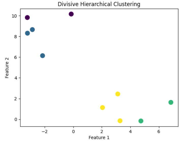
Final Clusters: [[2, 8], [7, 1, 4], [9, 6], [0, 3, 5]]

Step 7: Visualize the Result

Plot the clusters after divisive hierarchical clustering.

# Assign a cluster label to each point
labels = np.zeros(len(X))
for cluster_index, cluster in enumerate(clusters):
    for point in cluster:
        labels[point] = cluster_index

# Plot the clusters
plt.scatter(X[:, 0], X[:, 1], c=labels, cmap='viridis', s=100)
plt.title("Divisive Hierarchical Clustering")
plt.xlabel("Feature 1")
plt.ylabel("Feature 2")
plt.show()

OUTPUT:

Step-by-Step Explanation:

1. Import Required Libraries: Import libraries for matrix computation, distance calculation, and visualization.
2. Generate/Load Data: Create a dataset or load your real-world data for clustering.
3. Compute Distance Matrix: Calculate pairwise distances between all points using scipy.spatial.distance.pdist. This is used to determine dissimilarity.
4. Initialize a Single Cluster: Start with all points in one cluster, and represent clusters as a list of point indices.
5. Define Split Function: Identify the two most distant points in the cluster. Assign the rest of the points to the closer of these two points to form two subclusters.
6. Iteratively Split Clusters: At each step, choose the largest cluster and split it into two until the desired number of clusters is reached.
7. Visualize the Result: Plot the resulting clusters to understand how the algorithm has split the data.

Key Points:

• Stopping Criterion: The algorithm stops when the number of clusters equals the desired number or when the clusters cannot be split further.
• Distance Metric: You can change the distance metric (e.g., Manhattan or cosine) in the pdist function.
• Computational Complexity: Divisive clustering can be computationally expensive due to the distance matrix and recursive splitting.
  
  Next Blog- DBSCAN Clustering