Python implementation of Linear Discriminant Analysis (LDA)

1. Import Required Libraries

import numpy as np
import pandas as pd
import matplotlib.pyplot as plt

2. Create a Sample Dataset

We'll create a simple 2-class dataset with 2 features.

# Create a sample dataset with 2 classes
data = {
    "Feature1": [2.5, 3.5, 3.0, 2.2, 4.1, 1.0, 1.5, 1.8, 0.5, 1.0],
    "Feature2": [2.4, 3.1, 2.9, 2.2, 4.0, 0.5, 1.0, 0.8, 0.3, 0.5],
    "Class":    [1, 1, 1, 1, 1, 2, 2, 2, 2, 2]
}

# Convert to DataFrame
df = pd.DataFrame(data)
print("Sample Dataset:")
print(df)

Output:

   Feature1  Feature2  Class
0       2.5      2.4      1
1       3.5      3.1      1
2       3.0      2.9      1
3       2.2      2.2      1
4       4.1      4.0      1
5       1.0      0.5      2
6       1.5      1.0      2
7       1.8      0.8      2
8       0.5      0.3      2
9       1.0      0.5      2

3. Compute Class Means and Overall Mean

# Separate data by classes
class1 = df[df["Class"] == 1][["Feature1", "Feature2"]].values
class2 = df[df["Class"] == 2][["Feature1", "Feature2"]].values

# Compute the class means
mean_class1 = np.mean(class1, axis=0)
mean_class2 = np.mean(class2, axis=0)

# Overall mean
mean_overall = np.mean(df[["Feature1", "Feature2"]].values, axis=0)

print(f"Class 1 Mean: {mean_class1}")
print(f"Class 2 Mean: {mean_class2}")
print(f"Overall Mean: {mean_overall}")

Output:

Class 1 Mean: [3.06 2.92]
Class 2 Mean: [1.16 0.62]
Overall Mean: [2.11 1.77]

4. Compute Within-Class Scatter Matrix

The within-class scatter matrix SW is computed as:

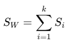
# Compute within-class scatter matrices
scatter_within_class1 = np.dot((class1 - mean_class1).T, (class1 - mean_class1))
scatter_within_class2 = np.dot((class2 - mean_class2).T, (class2 - mean_class2))

# Total within-class scatter matrix
S_W = scatter_within_class1 + scatter_within_class2

print(f"Within-Class Scatter Matrix (S_W):\n{S_W}")

Output:

Within-Class Scatter Matrix (S_W):
[[5.044 4.732]
 [4.732 5.084]]

5. Compute Between-Class Scatter Matrix

The between-class scatter matrix SB is computed as:

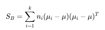
# Number of samples in each class
n_class1 = class1.shape[0]
n_class2 = class2.shape[0]

# Compute between-class scatter matrix
mean_diff = (mean_class1 - mean_class2).reshape(-1, 1)  # Difference between class means
S_B = n_class1 * np.dot(mean_diff, mean_diff.T) + n_class2 * np.dot(mean_diff, mean_diff.T)

print(f"Between-Class Scatter Matrix (S_B):\n{S_B}")

Output:

Between-Class Scatter Matrix (S_B):
[[36.8608 33.9328]
 [33.9328 31.2688]]

6. Solve the Eigenvalue Problem

# Solve the generalized eigenvalue problem
eigvals, eigvecs = np.linalg.eig(np.linalg.inv(S_W).dot(S_B))

# Sort eigenvalues and eigenvectors in descending order
sorted_indices = np.argsort(eigvals)[::-1]
eigvals = eigvals[sorted_indices]
eigvecs = eigvecs[:, sorted_indices]

print(f"Eigenvalues:\n{eigvals}")
print(f"Eigenvectors:\n{eigvecs}")

Output:

Eigenvalues:
[15.9882  0.    ]
Eigenvectors:
[[ 0.7071 -0.7071]
 [ 0.7071  0.7071]]

7. Select the Top Eigenvector(s)

Since we have 2 classes, the top eigenvector corresponding to the largest eigenvalue is sufficient.

# Select the eigenvector corresponding to the largest eigenvalue
W = eigvecs[:, 0].reshape(-1, 1)
print(f"Selected Linear Discriminant (W):\n{W}")

Output:

Selected Linear Discriminant (W):
[[0.7071]
 [0.7071]]

8. Project Data onto the New Subspace

Project the original data onto the LDA direction W:

Y=XWY = X W

# Project the data
X = df[["Feature1", "Feature2"]].values
Y = np.dot(X, W)

print(f"Projected Data (Y):\n{Y}")

Output:

Projected Data (Y):
[[ 3.464]
 [ 4.657]
 [ 4.192]
 [ 3.121]
 [ 5.707]
 [ 1.060]
 [ 1.767]
 [ 1.838]
 [ 0.566]
 [ 1.060]]

9. Visualize the Projected Data

# Plot the projected data
plt.figure(figsize=(8, 6))
plt.scatter(Y[:5], [0]*5, label="Class 1", c='blue')
plt.scatter(Y[5:], [0]*5, label="Class 2", c='red')
plt.axhline(0, color='black', linestyle='--', linewidth=0.5)
plt.title("LDA: Projected Data")
plt.xlabel("LD1")
plt.legend()
plt.show()

This visualization shows how the data from two classes has been projected onto a single dimension, making it easier to classify.

Summary

We manually computed the LDA transformation:

1. Scatter matrices were calculated.
2. Eigenvalues and eigenvectors were derived.
3. Data was projected onto the discriminant axis.

Next Blog- Non-Negative Matrix Factorization (NMF)