Machine learning (ML) is an interdisciplinary field that allows systems to learn and make decisions from data. However, raw data cannot be directly fed into machine learning algorithms; it needs to be processed first to ensure its suitability for learning models. One crucial step in this data preparation is understanding the data types present in the dataset. Different types of data require specific handling techniques during preprocessing. This blog will guide you through the process of understanding data types in the context of machine learning.
1.1 Data Preprocessing in Machine Learning
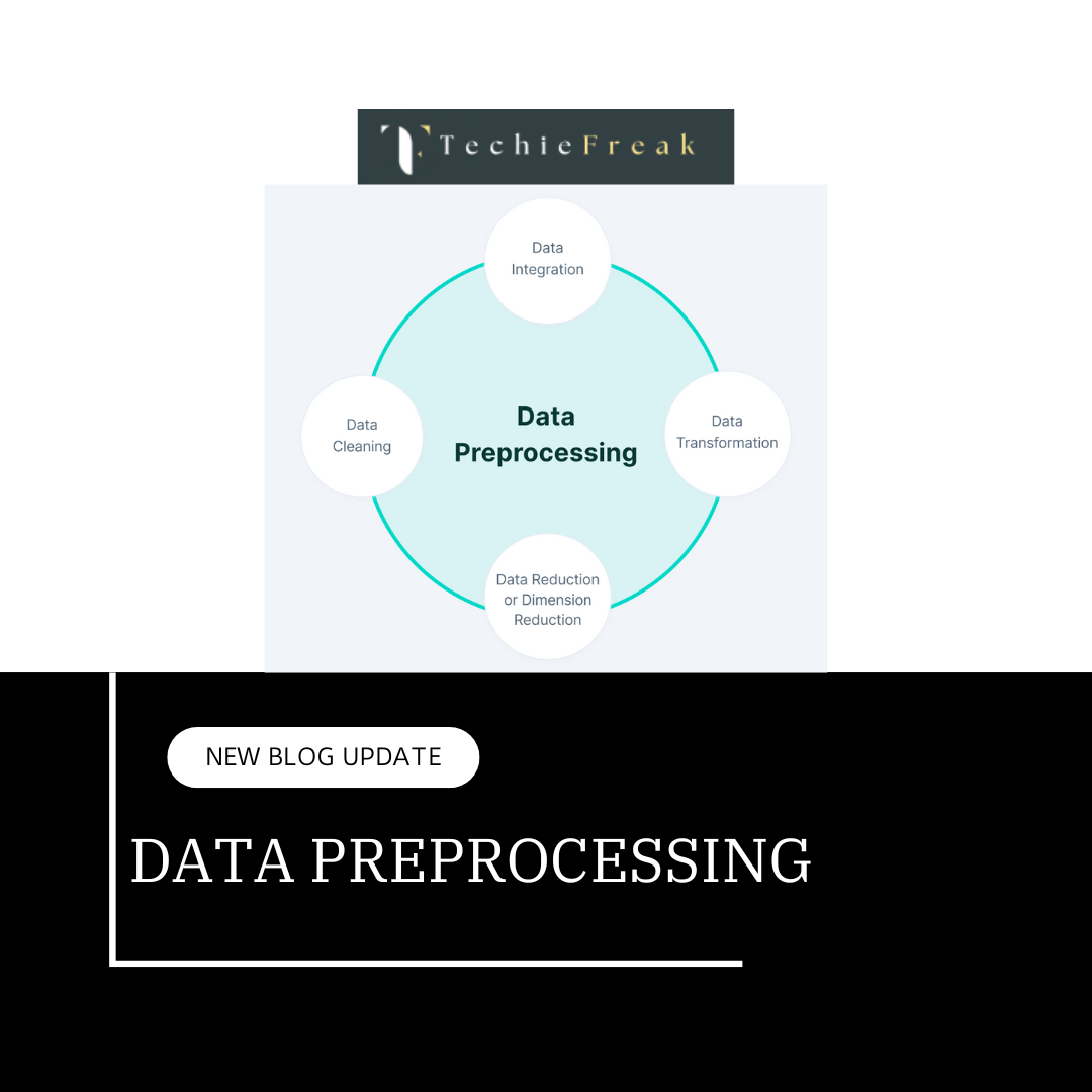
Data preprocessing refers to the process of cleaning, transforming, and organizing raw data into a format that machine learning algorithms can interpret. This process involves several steps, such as:
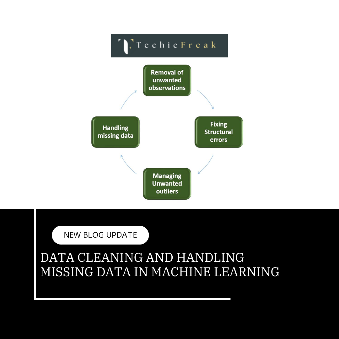
- Cleaning: Removing noise, handling missing values, and correcting errors.
- Transformation: Converting data into the appropriate format or structure for ML models.
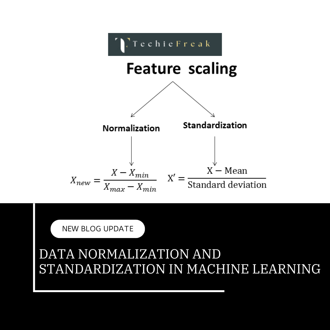
- Normalization/Standardization: Scaling features to bring uniformity across datasets.
- Encoding: Transforming categorical data into numeric forms for algorithmic processing.
However, before any of these steps can be done, it is essential to understand the types of data involved. Different data types come with unique challenges and preprocessing needs.
1.1.1 Understanding Data Types
1. Categorical Data
Categorical data, as mentioned, can be either nominal or ordinal. Let’s explore each type in greater detail.
Nominal Data
- Characteristics: Nominal data represents categories that don’t have any particular order or priority. These are simply labels, and the values cannot be ranked or compared in a meaningful way.
- Examples:
- Colors: Red, Blue, Green
- Product Categories: Electronics, Clothing, Groceries
- Gender: Male, Female, Non-binary
Handling Nominal Data:
To use nominal data in machine learning, we often convert it into numerical form:
- Label Encoding: Label encoding is a technique used to convert categorical data into numerical form. Each unique category is assigned a unique integer, making it possible for machine learning algorithms to process the data, as many models cannot handle categorical variables directly.
For instance:- Red → 0
- Blue → 1
- Green → 2
This is simple but might introduce a problem because machine learning models might interpret these numbers as having some order, which isn’t actually the case.
- One-Hot Encoding: One-hot encoding is a more widely-used method, particularly for nominal data. It converts each category into a binary vector (with 1s and 0s), indicating whether a particular category is present. For example:
- Color: Red → [1, 0, 0]
- Color: Blue → [0, 1, 0]
- Color: Green → [0, 0, 1]
Ordinal Data
- Characteristics: Ordinal data has a meaningful order, but the difference between the values is not uniform. For example, a rating system might have values such as "Bad", "Average", "Good", and "Excellent." While these labels have an inherent order, we cannot assume the difference between "Bad" and "Average" is the same as between "Good" and "Excellent."
- Examples:
- Movie ratings: Poor, Fair, Good, Excellent
- Education levels: High school, Bachelor's, Master's, PhD
Handling Ordinal Data:
Ordinal Encoding: Ordinal encoding is a technique used to transform categorical data into numerical values while preserving the inherent order among the categories. Unlike nominal data, ordinal data contains a natural sequence or ranking, but the difference between adjacent categories may not be uniform or meaningful.
For example:- Poor → 1
- Fair → 2
- Good → 3
- Excellent → 4
This ensures that the order is respected but doesn’t imply any uniform distance between the values.
- One-Hot Encoding: This can also be used for ordinal data, but it might result in losing the ordinal relationship between categories, so this approach is usually avoided for ordinal data unless required.
2. Numerical Data
Numerical data represents quantities that can be ordered and typically involves two types: discrete and continuous.
Discrete Data
- Discrete data refers to a type of quantitative data that consists of distinct and separate values. Unlike continuous data, which can take any value within a range, discrete data can only take specific values, typically integers, and cannot have fractions or decimals. This type of data is countable and often involves quantities that are whole numbers.
- Characteristics: Discrete data consists of distinct, countable values. These are often integers and don’t have any values in between.
- Examples:
- Number of children in a household
- Number of products sold
- Number of visits to a website
Handling Discrete Data:
For discrete numerical data, no transformation is usually needed, but you might need to:
- Handle Missing Values: Impute missing values using mean, median, or mode. For discrete data, median imputation might work better than mean imputation.
- Bin the Data: If the range of discrete data is very large (like the number of sales), it can be beneficial to create bins to group values together (e.g., sales in ranges of 0-10, 11-20, etc.).
Continuous Data
- Continuous data is a type of quantitative data that can take an infinite number of values within a given range. Unlike discrete data, which is countable and takes distinct values, continuous data represents measurements and can include fractions, decimals, or any value in between.
- Characteristics: Continuous data consists of infinite possible values within a range. These are typically real numbers (i.e., floats) and can represent anything from time to height, weight, or temperature.
- Examples:
- Age (e.g., 25.5 years)
- Height (e.g., 5.8 feet)
- Temperature (e.g., 72.5°F)
Handling Continuous Data:
- Normalization/Scaling: Continuous data often requires normalization or scaling to ensure consistency across features:
- Min-Max Scaling: Transforms data to a range between 0 and 1.
Formula:

Z-Score Standardization: Transforms data to have a mean of 0 and a standard deviation of 1.
Formula:
Where μ\mu is the mean and σ\sigma is the standard deviation of the feature.
- Handling Outliers: For continuous variables, outliers can significantly affect model performance, especially when using models sensitive to scale (like linear regression). You can:
- Remove outliers based on a defined threshold or a statistical test.
- Use robust models that are less sensitive to outliers, such as tree-based methods.
3. Text Data
Text data is a unique and complex data type in machine learning, especially in natural language processing (NLP). It consists of unstructured data that needs specific techniques to be processed.
Tokenization:
Tokenization involves splitting text into words or subwords. A common approach is to use space as a delimiter, but punctuation and special characters can also be treated as individual tokens.
- Example: "Machine learning is fun!" → ['Machine', 'learning', 'is', 'fun']
Stopword Removal:
Stopwords are common words (like "the", "is", "at", etc.) that don’t contribute significant meaning to the analysis. Removing them reduces the dimensionality of the text data.
- Example: “The quick brown fox” → ['quick', 'brown', 'fox']
Vectorization:
To use text in machine learning, it must be converted into numerical data. This can be done using several techniques:
- Bag of Words (BoW): Each unique word in the text becomes a feature. The value of each feature is the frequency of the word in the text.
- Example: “I love machine learning” → {I:1, love:1, machine:1, learning:1}
- TF-IDF (Term Frequency - Inverse Document Frequency): This method adjusts for the frequency of common words in all documents. The idea is to give higher weight to words that appear frequently in a particular document but not across all documents, making them more significant.
Formula:

Word Embeddings:
Word embeddings, like Word2Vec, GloVe, and FastText, are more advanced methods that map words into dense vectors of real numbers, capturing semantic relationships between words. For instance, "king" - "man" + "woman" = "queen".
4. Date/Time Data
Date and time data is common in datasets related to time series, forecasting, or event tracking. This type of data needs to be properly parsed to extract meaningful features.
Handling Date/Time Data:
- Parsing Date/Time: Dates should be converted into a standard format (e.g., YYYY-MM-DD) to make it easier for models to process.
- Feature Engineering:
- Extract components like year, month, day, hour, minute, and weekday.
- Example: “2023-01-01 14:23:00” → Year: 2023, Month: 01, Day: 01, Hour: 14, Minute: 23, Weekday: Sunday
- Time Differences: Calculate the difference between two date-time points. This can be useful when predicting time-dependent outcomes, such as customer churn or product lifecycle.
Handling Time Zones:
When working with global data, you need to convert time zones to ensure consistency. It’s crucial to convert all timestamps to a single time zone (e.g., UTC) to avoid errors.
Key Takeaways
The handling of data types is a critical step in the data preprocessing pipeline. Each type of data—whether categorical, numerical, text, or time-related—requires distinct techniques to prepare it for use in machine learning models. By carefully understanding and applying the right preprocessing methods for each data type, you can significantly improve the performance and accuracy of your models. Proper preprocessing also ensures that your machine learning algorithms will interpret your data in the way it was intended, leading to more meaningful predictions and insights.
Next Topic : Data cleaning and handling missing data
.png)
.png)
.png)
.png)
.png)
.png)
.png)
.png)
.png)
.png)
.png)
.png)
.png)
.png)
.png)
.png)
.png)
.png)
.png)
.png)
