Building a Machine Learning Pipeline
A Machine Learning (ML) pipeline is a systematic and automated process that streamlines the entire workflow of a machine learning project. It ensures efficiency, scalability, and reproducibility from data collection to model deployment and monitoring. This blog will walk you through the key stages involved in building an ML pipeline.
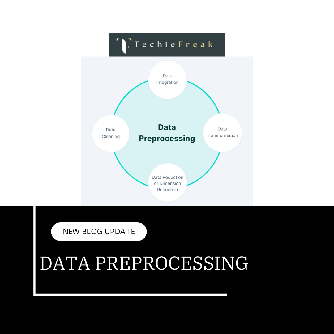
1. Data Collection and Preprocessing
The first step in any ML pipeline is gathering, cleaning, and transforming data into a usable format.
Building a Machine Learning Pipeline
a) Data Collection
Data collection is the first step in building a machine learning pipeline. High-quality data is crucial for training reliable models. Data can come from multiple sources, including:
- Databases (SQL, NoSQL, Data Warehouses)
- SQL Databases: Structured data stored in relational databases like MySQL, PostgreSQL, and Microsoft SQL Server. Data retrieval is done using SQL queries.
- NoSQL Databases: Unstructured or semi-structured data stored in databases like MongoDB, Firebase, and Cassandra. These are suitable for handling large-scale, flexible datasets.
- Data Warehouses: Centralized repositories like Google BigQuery, Amazon Redshift, and Snowflake that store large volumes of structured data optimized for analytics.
- APIs (REST, GraphQL)
- REST APIs: Representational State Transfer APIs provide access to data using HTTP methods like GET, POST, PUT, and DELETE. They return responses in JSON or XML format.
- GraphQL APIs: A more flexible query language for APIs that allows clients to request specific data fields instead of entire datasets. Useful for retrieving data efficiently.
- Examples: Twitter API for social media data, OpenWeather API for weather data, and Google Maps API for geolocation data.
- Web Scraping (BeautifulSoup, Scrapy)
- BeautifulSoup: A Python library for parsing HTML and XML documents to extract specific data points.
- Scrapy: A powerful web crawling framework that automates the scraping of large-scale datasets from websites.
- Examples: Scraping e-commerce sites for product prices, collecting news articles from online publications, and extracting stock market data from financial websites.
- Sensor Data (IoT Devices)
- Types of Sensors: Temperature sensors, accelerometers, gyroscopes, GPS trackers, heart rate monitors, and smart home devices.
- Data Transmission: Sensor data is transmitted using protocols such as MQTT (Message Queuing Telemetry Transport) and HTTP to cloud platforms like AWS IoT, Google Cloud IoT, and Azure IoT Hub.
- Examples: Smart thermostats collecting temperature data, fitness trackers monitoring physical activity, and autonomous vehicles gathering environmental information.
- Public Datasets (Kaggle, UCI Machine Learning Repository)
- Kaggle Datasets: Kaggle provides a vast collection of curated datasets, including those for image classification, NLP, financial analysis, and more.
- UCI Machine Learning Repository: A comprehensive collection of datasets widely used in research and academia for benchmarking machine learning models.
- Other Sources: Government portals (data.gov), WHO data repositories, Google Dataset Search, and academic research papers often provide open datasets for machine learning applications.
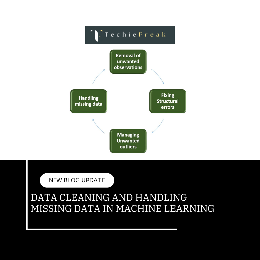
b) Data Cleaning
Raw data often contains errors and inconsistencies, which need to be handled to improve the quality and reliability of the dataset. Data cleaning involves several key steps:
- Removing Duplicates
- Duplicate records can occur due to multiple data collection processes or errors in merging datasets.
- Techniques:
- Using pandas' drop_duplicates() function in Python.
- Identifying duplicates based on unique identifiers or a combination of key fields.
- Removing unnecessary redundancy to improve model efficiency.
- Handling Missing Values
- Missing values can lead to incorrect model predictions and must be handled properly.
- Methods:
- Imputation: Filling missing values with mean, median, or mode.
- Forward/Backward Filling: Using previous or next available values to fill missing data in time-series datasets.
- Dropping Missing Data: Removing records or columns with excessive missing values.
- Predictive Imputation: Using machine learning algorithms to predict missing values based on other features.
- Correcting Inconsistent or Erroneous Values
- Errors in data entry, measurement mistakes, or system faults can introduce inconsistencies.
- Techniques:
- Standardizing categorical values (e.g., converting "NY" and "New York" to a consistent format).
- Correcting typos and misspellings using regex or NLP-based approaches.
- Ensuring numerical values fall within expected ranges (e.g., age should not be negative).
- Dealing with Outliers
- Outliers can distort model training and predictions.
- Methods:
- Statistical Approaches: Identifying outliers using Z-score, IQR (Interquartile Range), or box plots.
- Transformation Techniques: Applying log transformations or winsorizing data.
- Removing Outliers: If they result from data errors, they can be removed to enhance model performance.
- Capping: Setting threshold values to limit extreme values from affecting the model.
- Standardizing Data Formats
- Ensuring uniform data formatting, such as date formats, numerical precision, and categorical encodings.
- Examples:
- Converting all date fields to a consistent format (YYYY-MM-DD).
- Standardizing currency values and measurements (e.g., meters vs. feet).
- Handling Categorical Data
- Machine learning models often require categorical data to be converted into numerical form.
- Methods:
- Label Encoding: Assigning unique numbers to categorical values.
- One-Hot Encoding: Creating binary columns for each category to avoid ordinal relationships.
- Frequency Encoding: Replacing categories with their frequency counts.
Proper data cleaning enhances data integrity, reduces errors, and ensures that machine learning models perform optimally. The next step in the pipeline involves feature engineering and transformation.
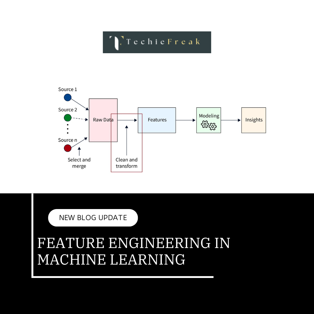
c) Feature Engineering
Feature engineering involves transforming raw data into meaningful input features to improve model performance:
- Feature extraction: Creating new variables from existing data to highlight important patterns. Examples include:
- Extracting date-related features (day, month, year, weekday) from timestamps.
- Converting text into numerical representations (TF-IDF, word embeddings).
- Generating statistical summaries (mean, variance, min-max) from groups of data.
- Feature selection: Identifying and retaining only the most relevant features to reduce dimensionality and improve model efficiency. Techniques include:
- Removing highly correlated features to avoid redundancy.
- Using algorithms like Recursive Feature Elimination (RFE) or mutual information for selection.
- Encoding categorical variables: Many machine learning algorithms require categorical data to be converted into numerical values. Common methods include:
- One-Hot Encoding: Creating binary columns for each category (suitable for nominal variables with a limited number of categories).
- Label Encoding: Assigning numerical labels to categories (useful for ordinal variables where order matters).
- Creating interaction features: Combining existing features to create new ones that capture relationships within the data. Examples include:
- Multiplying or adding numerical features to create interaction terms.
- Using polynomial features to capture non-linear relationships.
- Encoding domain-specific knowledge into features (e.g., calculating customer lifetime value in e-commerce data).
Effective feature engineering significantly impacts model performance by enhancing its ability to recognize patterns in data.
2. Data Splitting and Transformation
Before training a model, the dataset needs to be split and transformed appropriately.
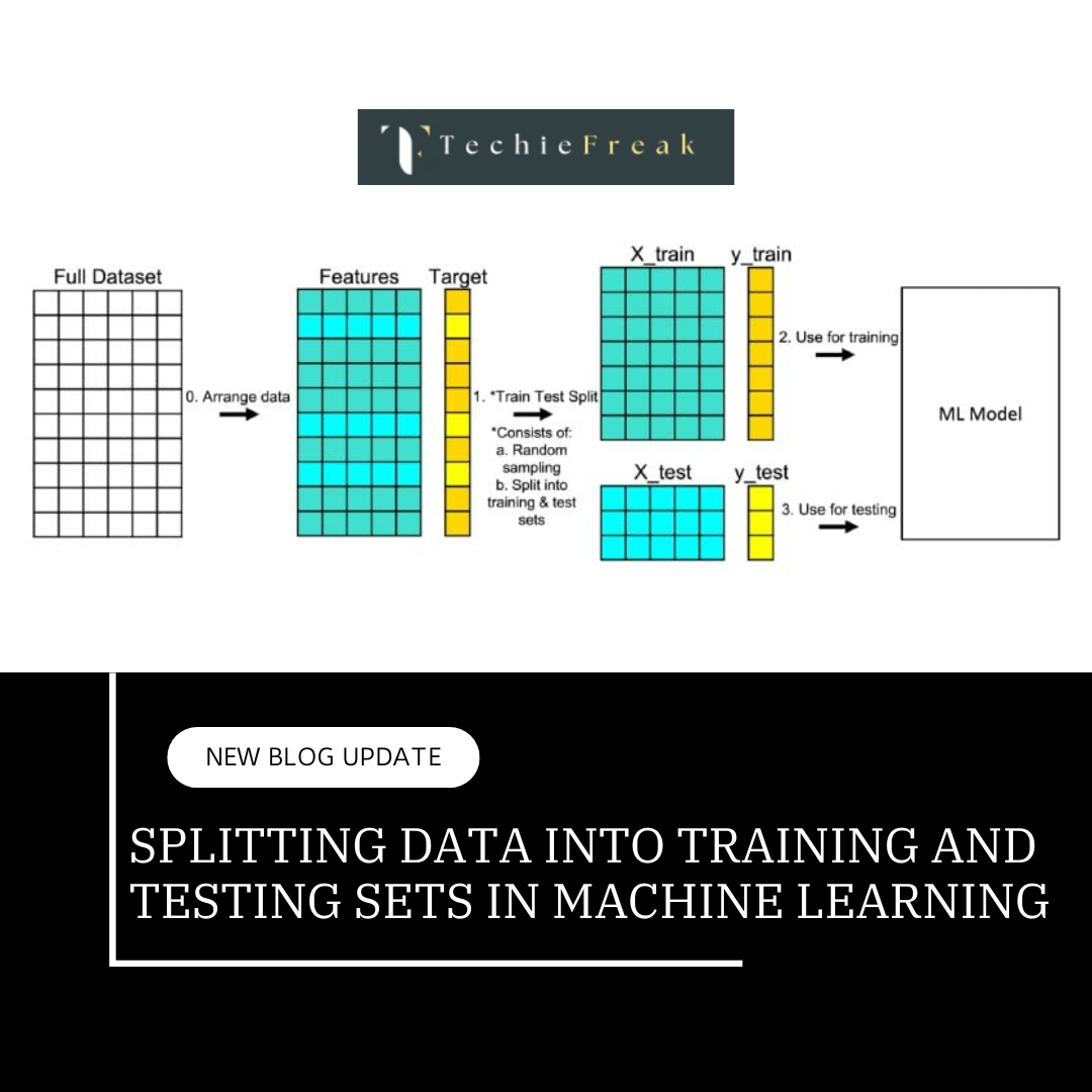
a) Data Splitting
Data splitting is a crucial step in machine learning, ensuring that a model is trained effectively and evaluated properly to avoid overfitting. It involves dividing the dataset into three parts:
- Training Set (70-80%)
- This portion of the data is used to train the machine learning model.
- The model learns patterns, relationships, and features from this data.
- It helps in optimizing the internal parameters of the model.
- Validation Set (10-15%)
- Used to fine-tune the model by adjusting hyperparameters (e.g., learning rate, number of layers in a neural network).
- Helps in preventing overfitting by ensuring the model generalizes well to unseen data.
- The model does not learn from this data, but its performance here guides hyperparameter selection.
- Test Set (10-15%)
- Used for final evaluation after the model has been trained and tuned.
- Measures the model's real-world performance on completely unseen data.
- Helps in assessing generalization ability before deployment.
Why Split Data?
- Prevents data leakage (where the model accidentally learns from future information).
- Ensures that the model generalizes well to new data.
- Helps in identifying overfitting (when the model performs well on training data but poorly on new data).
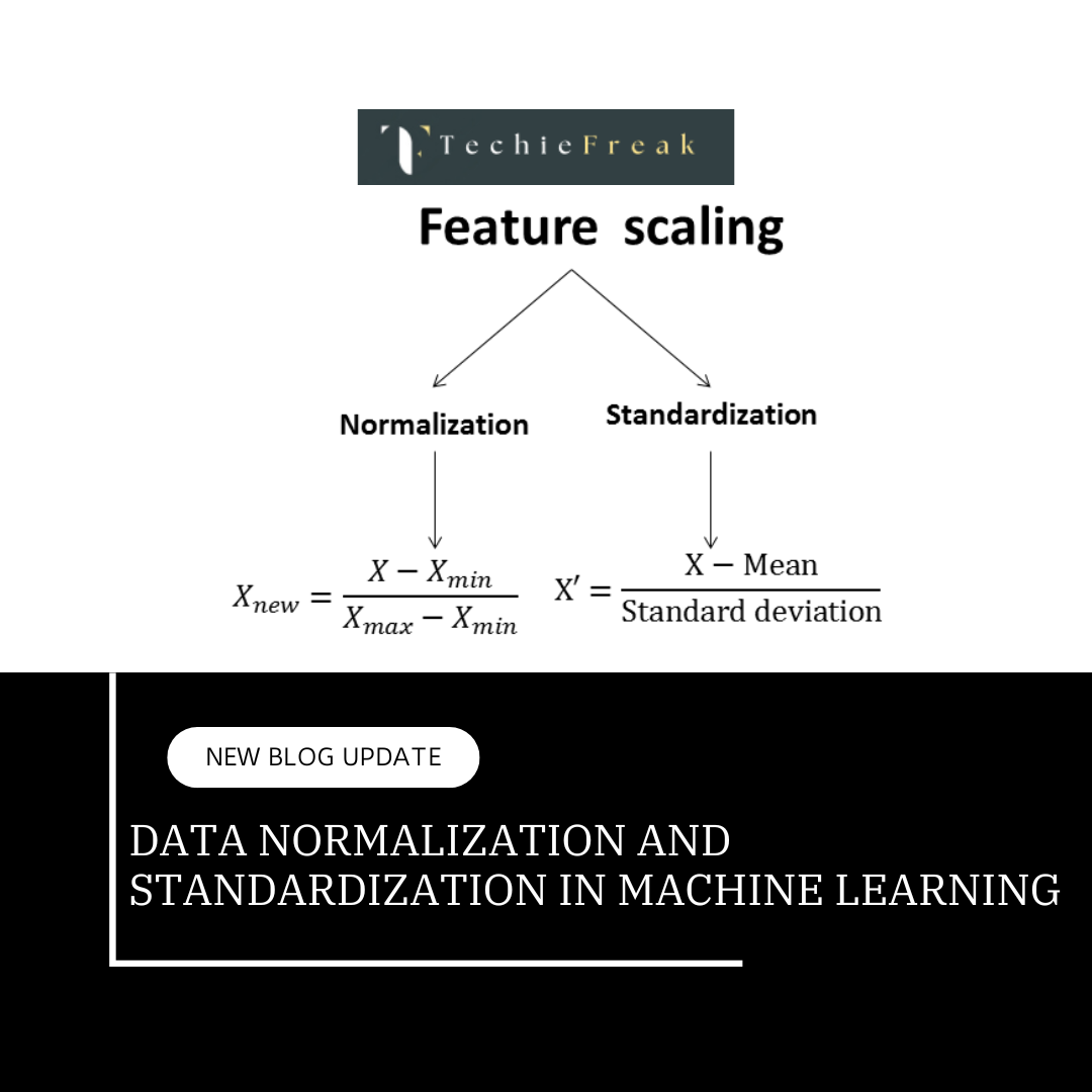
b) Data Normalization and Standardization
Machine learning algorithms perform better when numerical data is on a uniform scale:
Standardization (Z-score normalization):
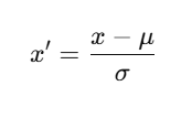
Where:
- x = original value
- μ = mean of the feature
σ = standard deviation of the feature
Explanation:
- Centers the data around mean = 0 with a standard deviation = 1.
- Keeps the shape of the original distribution but shifts and scales it.
- Works well for algorithms like SVM, k-Means, and PCA that assume data is normally distributed.
Normalization (Min-Max scaling):
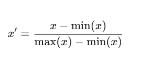
Where:
- x = original value
- min(x) = minimum value in the feature
max(x) = maximum value in the feature
Explanation:
- Scales data between 0 and 1 (or any custom range).
- Useful when feature values have different ranges.
- Works well for deep learning models and gradient-based algorithms (like neural networks and kNN).
3. Model Selection and Training
The next step is selecting an appropriate algorithm and training the model.
a) Choosing the Right Algorithm
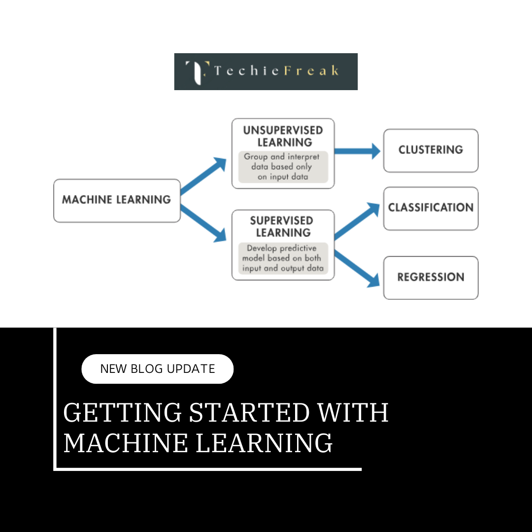
Selecting the right machine learning algorithm depends on the type of problem you are solving. It can be broadly categorized into Regression, Classification, Clustering, and Deep Learning.
1. Regression – Predicting Continuous Values
Regression algorithms are used when the target variable is a continuous numeric value.
Common Algorithms:
- Linear Regression – Works well when there is a linear relationship between variables.
- Decision Trees – Captures non-linear relationships but can overfit on small datasets.
- Random Forest – An ensemble of decision trees that improves accuracy and reduces overfitting.
Example: Predicting house prices based on factors like location, size, and number of rooms.
2. Classification – Predicting Categories
Classification is used when the target variable belongs to a set of predefined categories.
Common Algorithms:
- Logistic Regression – Best for binary classification problems.
- Support Vector Machine (SVM) – Works well with small datasets and finds an optimal decision boundary.
- Neural Networks – Useful for capturing complex patterns but requires large amounts of data.
Example: Identifying whether an email is spam or not based on text patterns.
3. Clustering – Grouping Similar Data (Unsupervised Learning)
Clustering algorithms group similar data points when there are no predefined labels.
Common Algorithms:
- K-Means – Partitions data into a specified number of clusters.
- DBSCAN – Works well for datasets with noise and clusters of varying sizes.
- Hierarchical Clustering – Builds a tree-like structure to represent relationships between clusters.
Example: Grouping customers based on shopping behavior to create targeted marketing strategies.
4. Deep Learning – Handling Complex Data (Images, Text, Time-Series)
Deep learning is used for highly complex problems where traditional machine learning may not be sufficient.
Common Architectures:
- Convolutional Neural Networks (CNNs) – Designed for image recognition and processing.
- Recurrent Neural Networks (RNNs) – Suitable for time-series and sequential data analysis.
Example: Detecting objects in an image or predicting future stock prices based on historical data.
How to Choose the Right Algorithm?
| Problem Type | Recommended Algorithms |
|---|---|
| Regression | Linear Regression, Decision Trees, Random Forest |
| Classification | Logistic Regression, SVM, Neural Networks |
| Clustering | K-Means, DBSCAN, Hierarchical Clustering |
| Image Processing | CNNs |
| Time-Series Data | RNNs, LSTMs |
b) Training the Model
Training a machine learning model involves improving its performance by adjusting internal parameters (weights) using training data. This process includes data batching, optimization techniques like gradient descent, and regularization methods to prevent overfitting.
1. Splitting Data into Batches
When training a model, instead of feeding all data at once, it is split into smaller batches to improve efficiency.
Why Use Batches?
- Reduces memory usage, especially for large datasets.
- Stabilizes learning by averaging updates over multiple examples.
- Speeds up training by allowing parallel computations.
Batching Methods:
Batch Training (Full-Batch Training)
- Uses the entire dataset for each update.
- More stable but computationally expensive.
- Suitable for small datasets.
Mini-Batch Training (Most Common Approach)
- Splits data into smaller batches (e.g., 32, 64, or 128 samples per batch).
- Balances efficiency and stability.
- Commonly used in deep learning.
Stochastic Gradient Descent (SGD)
- Updates model weights after processing each individual sample.
- Faster but results in more noise and fluctuations in training.
- Works well when training on very large datasets.
Example: Instead of processing 1 million images at once, they can be divided into mini-batches of 64 images each, making training feasible.
2. Optimizing Model Weights Using Gradient Descent
Gradient descent is the core optimization algorithm used to minimize the model’s error (loss function). It adjusts the model's weights to improve predictions.
How It Works:
- Compute the model’s error (loss) using the current weights.
- Calculate the gradient (direction of steepest descent).
- Update the weights in the opposite direction to reduce the error.
- Repeat until the error is minimized.
Types of Gradient Descent:
Batch Gradient Descent – Uses the entire dataset to compute updates, making it stable but slow.
Stochastic Gradient Descent (SGD) – Updates weights after each data point, making it faster but noisier.
Mini-Batch Gradient Descent – Updates weights after processing a mini-batch, balancing speed and stability.
Example: Training a neural network to recognize handwritten digits, adjusting weights after each batch of images.
3. Regularization Techniques (Preventing Overfitting)
Overfitting happens when a model learns patterns too specific to the training data, failing to generalize to new data. Regularization helps by adding constraints to the model.
Common Regularization Methods:
L1 Regularization (Lasso Regression)
- Adds a penalty proportional to the absolute value of weights (|w|).
- Helps in feature selection by shrinking some weights to zero, effectively removing unnecessary features.
L2 Regularization (Ridge Regression)
- Adds a penalty proportional to the square of weights (w²).
- Encourages smaller weights, making the model more stable.
- Commonly used in neural networks as weight decay.
Dropout (Used in Deep Learning)
- Randomly drops neurons during training to force the model to learn robust features.
Example: In image classification, L2 regularization prevents the model from memorizing specific pixel patterns, ensuring better generalization.
| Step | Purpose | Common Methods |
|---|---|---|
| Batching | Efficient training | Mini-Batch Training, Full-Batch Training, SGD |
| Optimization | Adjusting weights to reduce error | Gradient Descent (Batch, Mini-Batch, SGD) |
| Regularization | Preventing overfitting | L1 (Lasso), L2 (Ridge), Dropout |
c) Hyperparameter Tuning
Hyperparameters are predefined settings that control the behavior of a machine learning model. Unlike model parameters (such as weights in neural networks), hyperparameters are set before training and directly impact the model’s performance.
Hyperparameter tuning is the process of optimizing these settings to achieve the best results.
1. What Are Hyperparameters?
Hyperparameters vary based on the type of model used. Some common hyperparameters include:
- Learning Rate (η) – Controls how much the model updates weights during training.
- Number of Trees (for Random Forest, XGBoost) – Defines how many decision trees the ensemble method should use.
- Number of Hidden Layers and Neurons (for Neural Networks) – Determines the depth and size of the network.
- Regularization Strength (L1, L2 penalties) – Prevents overfitting by adding constraints to model weights.
- Batch Size – Defines how many samples are processed before updating model parameters.
Since hyperparameters are not learned from the data, choosing the right values requires experimentation.
2. Methods for Hyperparameter Tuning
To find the best hyperparameter combination, different search techniques are used:
1. Grid Search
How it works:
- Defines a set of possible values for each hyperparameter.
- Tests every possible combination to find the best performing set.
Pros:
- Guarantees finding the best combination (if included in the search space).
- Simple and easy to implement.
Cons:
- Computationally expensive, especially with large datasets.
- Inefficient if many parameter values do not significantly impact performance.
Example:
If tuning a Support Vector Machine (SVM), a grid search might test different combinations of:
- Kernel: {linear, polynomial, RBF}
- Regularization parameter (C): {0.1, 1, 10}
- Gamma: {0.01, 0.1, 1}
This would require testing 3 × 3 × 3 = 27 different models.
2. Random Search
How it works:
- Instead of testing all combinations, it selects random hyperparameter values within a given range.
- Runs a fixed number of random trials.
Pros:
- Faster than grid search since it does not check all possible values.
- Often finds good hyperparameter settings with fewer trials.
Cons:
- No guarantee of finding the optimal combination.
- Requires a well-defined range of hyperparameter values.
Example:
Instead of checking every combination of learning rates and batch sizes, a random search might try 10 random values, covering a broader range without testing all possibilities.
3. Bayesian Optimization
How it works:
- Uses past evaluations to predict the best next set of hyperparameters.
- Builds a probabilistic model of the objective function and refines its search based on previous results.
Pros:
- More efficient than grid and random search, requiring fewer trials.
- Learns from past evaluations to improve future selections.
Cons:
- More complex to implement.
- Requires additional computation for building probabilistic models.
Example:
Instead of randomly trying hyperparameters, Bayesian Optimization fits a model (such as a Gaussian process) to estimate which hyperparameter set is most likely to perform well.
Comparison of Hyperparameter Tuning Methods
| Method | Efficiency | Computational Cost | Best Use Case |
|---|---|---|---|
| Grid Search | High (tests all combinations) | Very High | Small datasets with a limited number of hyperparameters |
| Random Search | Medium (samples randomly) | Medium | Large hyperparameter spaces where full search is impractical |
| Bayesian Optimization | High (uses past evaluations) | Medium-High | Expensive models where fewer evaluations are preferred |
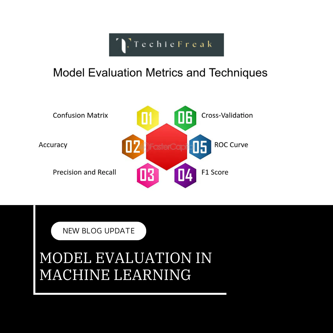
4. Model Evaluation
Evaluating a machine learning model is crucial to ensure that it generalizes well to unseen data. A good model should not only perform well on training data but also make accurate predictions on new inputs.
a) Key Performance Metrics
Different types of machine learning problems require different evaluation metrics.
Regression Metrics
Regression models predict continuous values (e.g., predicting house prices or temperature).
- Mean Squared Error (MSE)
- Measures the average squared difference between predicted and actual values.
Formula:

- Lower MSE values indicate better model performance.
- R-Squared Score (R² or Coefficient of Determination)
- Measures how well the model explains the variance in the data.
Formula:

- R² ranges from 0 to 1, where 1 means perfect predictions and 0 means the model explains no variance in the data.
Classification Metrics
Classification models predict discrete labels (e.g., spam vs. not spam, fraud detection).
- Accuracy
- Measures the percentage of correctly predicted labels.
Formula:

- Works well for balanced datasets, but not for imbalanced ones.
- Precision
- Measures the proportion of correctly identified positive instances out of all predicted positives.
Formula:

- Important for scenarios where false positives are costly (e.g., medical diagnosis).
- Recall (Sensitivity or True Positive Rate)
- Measures the proportion of actual positives correctly identified.
Formula:

- Important for cases where false negatives are costly (e.g., fraud detection).
- F1-Score
- The harmonic mean of precision and recall, balancing both metrics.
Formula:

- Useful when dealing with imbalanced datasets.
- ROC-AUC (Receiver Operating Characteristic - Area Under Curve)
- Measures the ability of a classifier to distinguish between classes at various threshold settings.
- Higher AUC values indicate a better model.
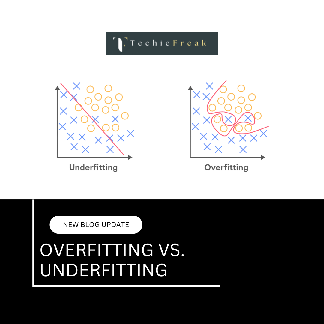
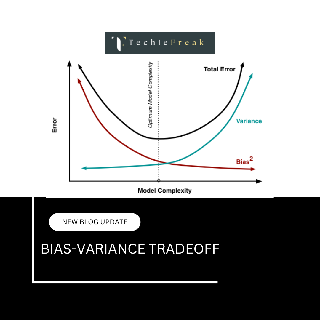
b) Overfitting and Underfitting
Overfitting
- Happens when a model memorizes training data but fails on new data.
- Signs of overfitting:
- High training accuracy but low test accuracy.
- Model captures noise instead of actual patterns.
- Causes:
- Too many parameters (complex model).
- Small dataset with high variance.
- Solutions:
- Use more training data.
- Apply regularization techniques (L1, L2).
- Use dropout (for deep learning models).
- Reduce model complexity (fewer layers, pruning decision trees).
Underfitting
- Happens when a model is too simple and fails to capture patterns in the data.
- Signs of underfitting:
- Low training accuracy and low test accuracy.
- High bias (wrong assumptions about data).
- Causes:
- Model is too simple (e.g., using linear regression for non-linear data).
- Not enough features.
- Too much regularization.
- Solutions:
- Use a more complex model (e.g., switch from linear regression to polynomial regression).
- Increase training time.
- Use better features (feature engineering).
5. Model Optimization and Fine-Tuning
To improve model performance, several techniques can be applied:
- Feature importance analysis (identifying significant features)
- Hyperparameter tuning (adjusting learning rate, batch size, regularization)
- Ensemble methods (combining multiple models for better predictions)
- Bagging (Random Forests)
- Boosting (Gradient Boosting, XGBoost, AdaBoost)
6. Model Deployment
After training and optimizing a machine learning model, the next step is deployment—making the model accessible for real-world applications. Deployment ensures that users or systems can interact with the model to make predictions, automate tasks, or integrate it into existing workflows.
a) Model Serialization
Before deployment, the trained model needs to be saved in a format that allows it to be reloaded and used later. This process is called model serialization.
Saving Models Locally
- Pickle (.pkl format)
- Used for saving and loading Python objects, including machine learning models.
- Suitable for small-scale projects.
Example:
import pickle
with open("model.pkl", "wb") as file:
    pickle.dump(model, file)
- Joblib
- More efficient than Pickle for saving large models (especially those with NumPy arrays).
Example:
import joblib
joblib.dump(model, "model.joblib")
Exporting for Large-Scale Deployment
For production-level deployment, more robust formats are used:
- ONNX (Open Neural Network Exchange Format)
- A universal format for ML models, enabling compatibility across frameworks.
- Useful for cross-platform deployment.
- TensorFlow Serving
- Used for serving TensorFlow models efficiently in production.
- Provides REST and gRPC endpoints for model predictions.
- TorchScript
- Used for exporting PyTorch models to run in production environments like C++ applications or mobile devices.
b) Deployment Options
Once the model is serialized, it can be deployed using different approaches, depending on the use case.
1. Deployment via REST APIs
- A machine learning model can be deployed as a REST API, allowing users or applications to send input data and receive predictions.
- Common frameworks for building ML APIs:
- FastAPI (lightweight and fast)
- Flask (simple and widely used)
- Django (robust for large applications)
Example: Deploying a model using FastAPI
from fastapi import FastAPI
import joblib
import numpy as np

app = FastAPI()
model = joblib.load("model.joblib")

@app.post("/predict/")
def predict(data: list):
    prediction = model.predict(np.array(data).reshape(1, -1))
    return {"prediction": prediction.tolist()}
2. Cloud Deployment
For large-scale applications, deploying models on the cloud provides scalability, security, and performance optimization.
Popular cloud platforms for ML model deployment:
- AWS SageMaker – Fully managed service for training, tuning, and deploying models.
- Google AI Platform – Deploys models on Google Cloud for real-time predictions.
- Azure Machine Learning – Microsoft's cloud service for ML deployment.
3. Edge Deployment
- In edge computing, models run directly on mobile devices, IoT devices, or embedded systems instead of cloud servers.
- Useful for applications where low latency and offline functionality are required (e.g., voice assistants, image recognition on phones).
- Tools for edge deployment:
- TensorFlow Lite – Optimized for mobile and embedded devices.
- CoreML – Apple’s framework for running ML models on iOS devices.
- ONNX Runtime – Runs optimized ML models on edge devices.
Example: Converting a TensorFlow model for mobile deployment
import tensorflow as tf

model = tf.keras.models.load_model("model.h5")
converter = tf.lite.TFLiteConverter.from_keras_model(model)
tflite_model = converter.convert()

with open("model.tflite", "wb") as file:
    file.write(tflite_model)
Read more - Deployment Options
7. Model Monitoring and Maintenance
After deploying a machine learning model, continuous monitoring and maintenance are essential to ensure that the model remains accurate, reliable, and efficient. Models can degrade over time due to changing data patterns, known as concept drift, or due to system failures.
a) Performance Tracking
Tracking model performance helps identify any degradation in accuracy, precision, recall, or other key metrics. This is done by logging predictions and evaluating the model's accuracy over time.
1. Logging Predictions and Accuracy Trends
- Keep a record of model predictions and compare them with actual outcomes.
- Track performance metrics like accuracy, precision, recall, F1-score, and Mean Squared Error (MSE).
- Maintain logs to analyze trends and detect performance drops.
2. Tools for Performance Tracking
Several tools help automate logging and visualization of model performance:
- MLflow – Tracks experiments, model parameters, and versioning.
- TensorBoard – Visualizes deep learning models, training loss, and accuracy trends.
- Prometheus – Monitors real-time data, collects time-series metrics, and sends alerts.
Example: Logging predictions with MLflow
import mlflow

mlflow.start_run()
mlflow.log_metric("accuracy", 0.92)
mlflow.log_param("learning_rate", 0.01)
mlflow.end_run()
b) Handling Concept Drift
1. What is Concept Drift?
Concept drift occurs when the statistical properties of the input data change over time, causing the model to become less effective. For example:
- A fraud detection model trained on past transactions might struggle with new fraudulent techniques.
- A stock price prediction model may lose accuracy due to market shifts.
2. Detecting Concept Drift
- Statistical Tests – Compare new data distributions with training data.
- Kolmogorov-Smirnov Test – Checks if the distribution of new data significantly differs from old data.
- Population Stability Index (PSI) – Measures how much a variable's distribution has changed.
Example: Using Kolmogorov-Smirnov test
from scipy.stats import ks_2samp

# Compare old vs new data distributions
stat, p_value = ks_2samp(old_data, new_data)

if p_value < 0.05:
    print("Concept drift detected! Model retraining needed.")
3. Retraining the Model
- Periodically retrain the model with fresh data.
- Use automated pipelines to schedule retraining at regular intervals.
- Implement online learning where the model continuously learns from new data.
Example: Auto-retraining with scikit-learn
from sklearn.model_selection import train_test_split

# Train a new model with updated data
X_train, X_test, y_train, y_test = train_test_split(new_data, labels, test_size=0.2)
model.fit(X_train, y_train)
c) Implementing Alerting Systems
1. Triggering Alerts for Anomalies
Anomalies in predictions (such as a sudden drop in accuracy or unexpected outputs) must trigger alerts so that issues can be addressed.
- Set accuracy thresholds – If accuracy drops below a certain level, trigger an alert.
- Detect outliers – Flag unexpected predictions.
- Use monitoring dashboards – Send alerts via Slack, email, or SMS.
Example: Setting an alert if accuracy falls below a threshold
accuracy = 0.75  # Current model accuracy
threshold = 0.80

if accuracy < threshold:
    print("Warning: Model accuracy has dropped! Consider retraining.")
2. Deploying Fail-Safe Mechanisms
- Rollback to previous model versions – If the new model underperforms, revert to an earlier version.
- Shadow Deployment – Test the new model alongside the old one before fully switching.
- A/B Testing – Deploy two models and compare results before selecting the best one.
Example: Using MLflow for model versioning
import mlflow

# Load a previous version of the model
model = mlflow.pyfunc.load_model("models:/fraud_detection/Production")
Read more - Model Monitoring and Maintenance
Key Takeaways
Building an end-to-end machine learning pipeline ensures efficiency, scalability, and maintainability. By following a systematic approach from data preprocessing to deployment and monitoring, ML models can be seamlessly integrated into real-world applications. Automating this pipeline reduces manual effort and accelerates the ML lifecycle, making AI-driven solutions more practical and impactful.
.png)
.png)
.png)
.png)
.png)
.png)
.png)
.png)
.png)
.png)
.png)
.png)
.png)
.png)
.png)
.png)
.png)
.png)
.png)
.png)
