Mastering DataFrame Operations in Pandas
Pandas is an essential library in Python for data manipulation and analysis. At the core of Pandas is the DataFrame, a 2D labeled data structure. Mastering DataFrame operations in Pandas is crucial for efficiently handling, cleaning, and analyzing data.
In this blog, we’ll dive deep into various DataFrame operations—from basic tasks like filtering and sorting to more advanced operations such as merging, reshaping, and applying functions to the data. We’ll cover practical examples and scenarios to demonstrate how to use these operations effectively.
Understanding the DataFrame in Pandas
A DataFrame is similar to a table or a spreadsheet. It has rows and columns, each identified by index and column labels respectively. It’s the most common and versatile data structure in Pandas. A DataFrame can contain data of various types (integers, floats, strings, etc.), and you can perform a wide range of operations on it.
Here’s an example of creating a simple DataFrame:
import pandas as pd

# Creating a DataFrame
data = {'Name': ['Alice', 'Bob', 'Charlie'],
        'Age': [25, 30, 35],
        'City': ['New York', 'Los Angeles', 'Chicago']}

df = pd.DataFrame(data)

print(df)
Output:
       Name  Age         City
0     Alice   25     New York
1       Bob   30  Los Angeles
2   Charlie   35      Chicago
In this DataFrame:
- The columns are 'Name', 'Age', and 'City'.
- The index is automatically created as 0, 1, 2 (but it can be customized).
1. Accessing Data in a DataFrame
To start working with a DataFrame, you need to access its data. There are several ways to do this:
Accessing Columns
You can access a column by using the column name as a key:
# Accessing a column
print(df['Name'])
Output:
0      Alice
1        Bob
2    Charlie
Name: Name, dtype: object
Accessing Rows
You can access rows using the iloc[] and loc[] methods:
- iloc[]: Integer-location based indexing for selecting by position.
- loc[]: Label-based indexing for selecting by index name.
# Accessing a row by position (index 0)
print(df.iloc[0])

# Accessing a row by label (index 'a' if available)
# print(df.loc[0])
Output for iloc:
Name      Alice
Age          25
City    New York
Name: 0, dtype: object
Accessing Multiple Rows and Columns
You can also access multiple rows or columns:
# Accessing multiple columns
print(df[['Name', 'Age']])

# Accessing multiple rows
print(df.iloc[0:2])  # Rows 0 and 1
2. Filtering Data in a DataFrame
Filtering allows you to extract subsets of data based on conditions.
Conditional Filtering
You can filter data based on conditions applied to columns:
# Filtering data where age is greater than 30
filtered_df = df[df['Age'] > 30]
print(filtered_df)
Output:
       Name  Age     City
2   Charlie   35  Chicago
Multiple Conditions
You can also filter using multiple conditions:
# Filtering data with multiple conditions
filtered_df = df[(df['Age'] > 20) & (df['City'] == 'New York')]
print(filtered_df)
Output:
    Name  Age      City
0  Alice   25  New York
3. Sorting Data in a DataFrame
Sorting allows you to arrange the rows of the DataFrame in a specified order based on one or more columns.
Sorting by a Single Column
# Sorting by Age in ascending order
sorted_df = df.sort_values(by='Age')
print(sorted_df)
Output:
       Name  Age         City
0     Alice   25     New York
1       Bob   30  Los Angeles
2   Charlie   35      Chicago
Sorting by Multiple Columns
# Sorting by multiple columns (Age then Name)
sorted_df = df.sort_values(by=['Age', 'Name'])
print(sorted_df)
Output:
       Name  Age         City
0     Alice   25     New York
1       Bob   30  Los Angeles
2   Charlie   35      Chicago
4. Adding, Modifying, and Dropping Columns
Adding a New Column
You can add new columns to a DataFrame by directly assigning values:
# Adding a new column 'Salary'
df['Salary'] = [50000, 60000, 70000]
print(df)
Output:
       Name   Age         City          Salary
0     Alice   25        New York        50000
1       Bob   30        Los Angeles     60000
2   Charlie   35        Chicago         70000
Modifying an Existing Column
You can modify the values of an existing column:
# Modifying the 'Salary' column
df['Salary'] = df['Salary'] * 1.1  # Increase salary by 10%
print(df)
Output:
       Name  Age         City  Salary
0     Alice   25     New York   55000.0
1       Bob   30  Los Angeles   66000.0
2   Charlie   35      Chicago   77000.0
Dropping a Column
To remove a column, you can use the drop() method:
# Dropping the 'Salary' column
df = df.drop(columns=['Salary'])
print(df)
Output:
       Name  Age         City
0     Alice   25     New York
1       Bob   30  Los Angeles
2   Charlie   35      Chicago
5. Grouping Data
Grouping data allows you to perform aggregate operations on subsets of data based on one or more columns.
# Grouping by 'City' and calculating average Age
grouped_df = df.groupby('City')['Age'].mean()
print(grouped_df)
Output:
City
Chicago         35.0
Los Angeles     30.0
New York        25.0
Name: Age, dtype: float64
6. Merging and Concatenating DataFrames
_1735032971.png)
Pandas allows you to combine multiple DataFrames using the merge() and concat() functions.
Merging DataFrames
# Merging two DataFrames based on a common column
df1 = pd.DataFrame({'ID': [1, 2], 'Name': ['Alice', 'Bob']})
df2 = pd.DataFrame({'ID': [1, 2], 'Age': [25, 30]})

merged_df = pd.merge(df1, df2, on='ID')
print(merged_df)
Output:
   ID   Name  Age
0   1  Alice   25
1   2    Bob   30
Concatenating DataFrames
# Concatenating DataFrames along rows
df3 = pd.DataFrame({'ID': [3], 'Name': ['Charlie'], 'Age': [35]})
concatenated_df = pd.concat([df1, df3])
print(concatenated_df)
Output:
   ID     Name  Age
0   1    Alice   25
1   2      Bob   30
2   3  Charlie   35
7. Applying Functions to DataFrames
You can apply functions to individual columns or rows using the apply() method.
# Applying a function to a column
df['Age_in_5_years'] = df['Age'].apply(lambda x: x + 5)
print(df)
Output:
       Name  Age         City  Age_in_5_years
0     Alice   25     New York              30
1       Bob   30  Los Angeles              35
2   Charlie   35      Chicago              40
Key Takeaways
- DataFrame Basics: A DataFrame is a two-dimensional, labeled data structure in Pandas, composed of rows and columns.
- Accessing Data: You can access data in a DataFrame using column names, iloc[] (by position), or loc[] (by label).
- Filtering: Use conditions and boolean indexing to filter rows and extract subsets of data.
- Sorting: Sort data using the sort_values() method, either by one or multiple columns.
- Modifying Data: You can add, modify, and drop columns in a DataFrame.
- Grouping: Use the groupby() method to perform aggregate operations on data.
- Merging and Concatenating: Combine DataFrames using merge() and concat().
- Applying Functions: Apply functions to columns or rows using the apply() method for more customized operations.
Next Topic : Grouping, Aggregating, and Merging Data in Pandas
.png)


.png)








.png)

