Introduction
Machine Learning (ML) is revolutionizing the world as we know it, powering everything from Netflix recommendations to self-driving cars. It’s a game-changer across industries like healthcare, finance, entertainment, and retail. But what exactly is Machine Learning, and how can you begin this exciting journey? In this guide, we’ll demystify the fundamentals, introduce you to the types of Machine Learning, and explore its real-world applications.
What is Machine Learning?
Machine Learning is a branch of Artificial Intelligence (AI) that allows computers to learn and make decisions based on data, without explicit programming. Unlike traditional coding—where rules are manually defined—ML algorithms uncover patterns from data and evolve with experience.
For instance, instead of coding rules to identify spam emails, an ML model learns from examples of spam and non-spam emails, identifying characteristics that distinguish the two.
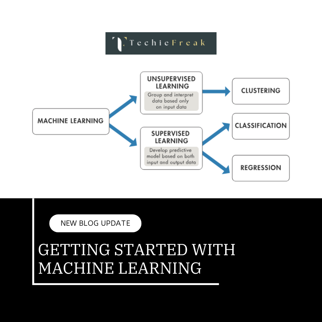
Types of Machine Learning
- Supervised Learning:
Supervised learning is akin to teaching a child with labeled examples. The algorithm learns from input-output pairs, where the “output” is already known. Once trained, it predicts outcomes for new, unseen inputs.
Example: Predicting house prices based on location, size, and other factors. - Unsupervised Learning:
This type of learning deals with unlabeled data. The model seeks patterns or structures within the data without predefined labels. It’s like organizing a messy room without knowing the categories in advance.
Example: Grouping customers with similar buying habits (customer segmentation). - Reinforcement Learning:
Reinforcement Learning involves an agent learning through interaction with an environment. The agent receives feedback in the form of rewards or penalties and adjusts its behavior to maximize rewards.
Example: AI mastering games like chess or training robots to navigate spaces.
Applications of Machine Learning
The impact of Machine Learning spans countless industries and daily activities. Let’s take a closer look:
- Healthcare: ML assists in early disease detection, medical imaging analysis, and personalized treatment plans.
Example: Predicting patient recovery times post-surgery. - Finance: Banks and fintech companies use ML for fraud detection, credit scoring, and portfolio optimization.
Example: Identifying unusual transaction patterns to prevent fraud. - Entertainment: Streaming platforms like Netflix and Spotify use ML to recommend movies and music based on your preferences.
Example: "You might like" recommendations. - Retail: Retailers optimize pricing strategies, manage inventory, and predict customer purchase behavior with ML models.
Example: Suggesting products frequently bought together. - Autonomous Vehicles: Self-driving cars rely on ML for recognizing traffic signs, detecting pedestrians, and planning optimal routes.
Key Terminology in Machine Learning:
As you step into the world of Machine Learning, understanding these foundational terms will help:
- Algorithm: The set of rules or steps used to process data and make predictions.
- Model: The mathematical structure created by training an algorithm on data.
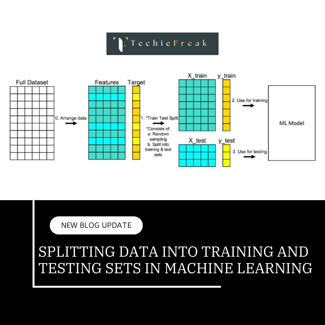
- Training Data: The dataset the algorithm learns from to build a model.
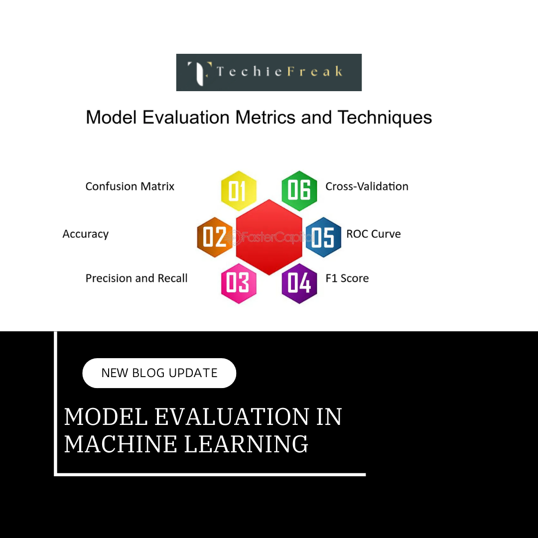
- Test Data: A separate dataset used to assess how well the model performs.
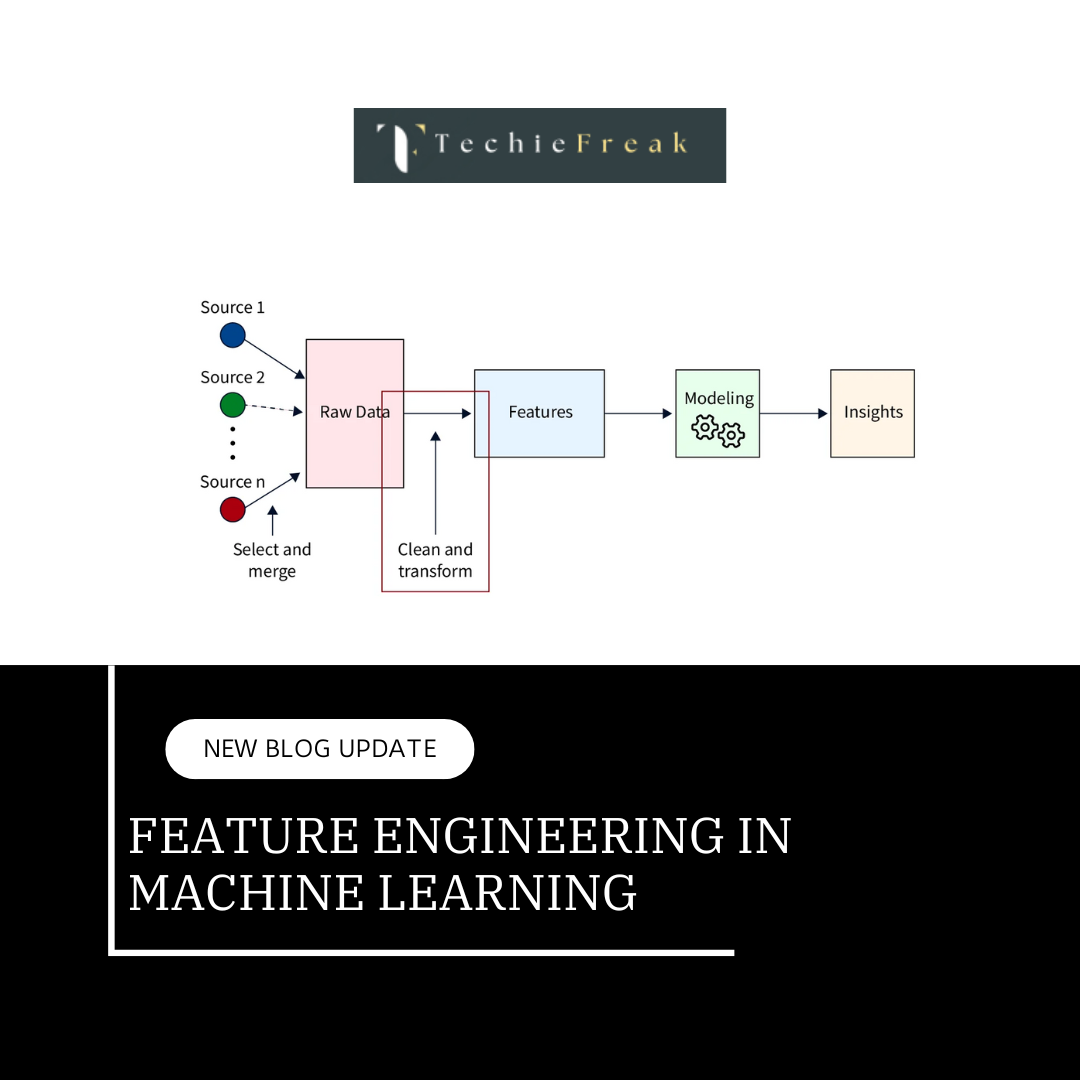
- Features: Input variables that influence the output (e.g., age, income, and education in predicting loan eligibility).
- Labels: The desired output or prediction (e.g., loan approved or not).
How to Begin Your Machine Learning Journey
Getting started in Machine Learning is simpler than you think. Follow these steps to build a strong foundation:
- Master Python Basics: Python is the go-to language for ML due to its simplicity and extensive library support. Start with Python syntax, loops, and functions.
- Understand Core Math Concepts: Strengthen your knowledge of linear algebra, statistics, and probability—they’re essential for understanding ML models.
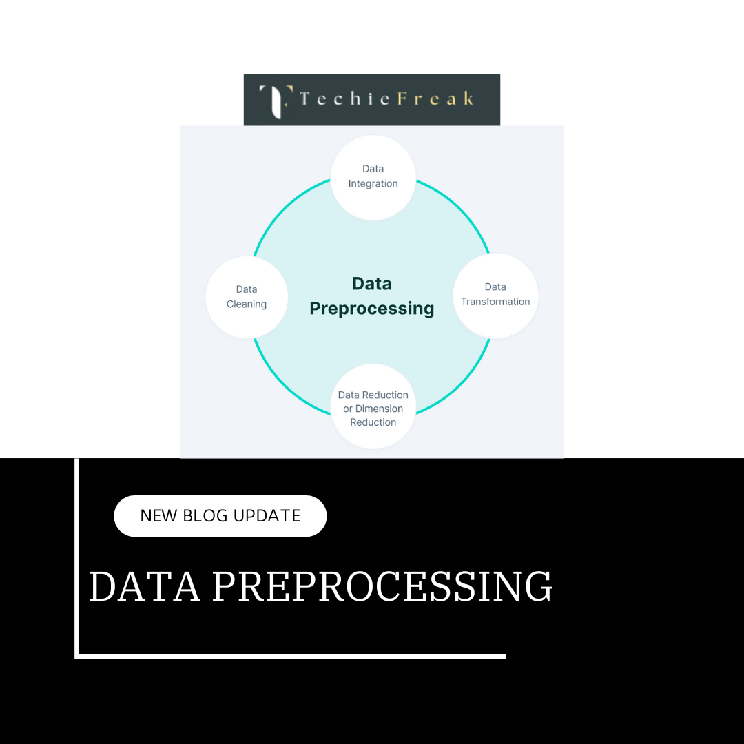
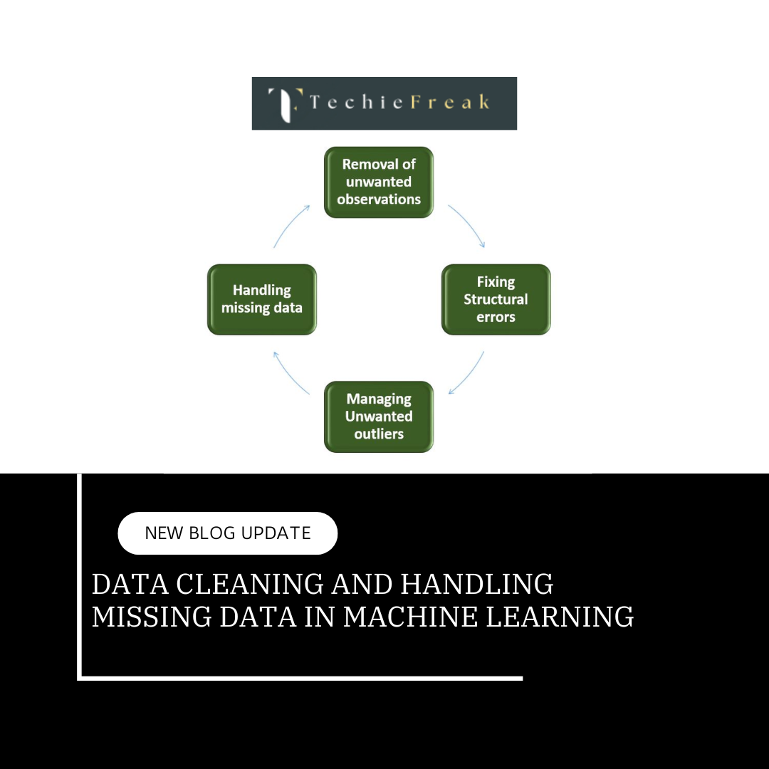
- Learn Data Preprocessing: Data is the fuel for ML. Practice cleaning, transforming, and normalizing data using Python libraries like Pandas.
- Experiment with Simple Algorithms: Start with foundational algorithms like linear regression or decision trees to grasp how predictions are made.
- Leverage ML Tools: Tools like Scikit-learn, TensorFlow, and PyTorch make implementing complex algorithms easier.
- Work on Real Datasets: Practice by solving Kaggle challenges or exploring publicly available datasets (e.g., Titanic dataset).
- Stay Curious and Consistent: Keep experimenting, learning, and building projects to strengthen your skills.
Conclusion
Machine Learning is an ever-evolving field that opens doors to countless possibilities. From creating impactful applications to solving real-world problems, the journey of becoming proficient in ML starts with mastering the basics.
In our next blog, we’ll focus on the basics of Python for Machine Learning — your essential toolkit for data manipulation, visualization, and building models.
Ready to take the next step? Stay tuned!


.png)
.png)
.png)
.png)
.png)
.png)
.png)
.png)
.png)
.png)
.png)
.png)
.png)
.png)
.png)
.png)
.png)
.png)
.png)
.png)