Python Implementation of Agglomerative Hierarchical Clustering

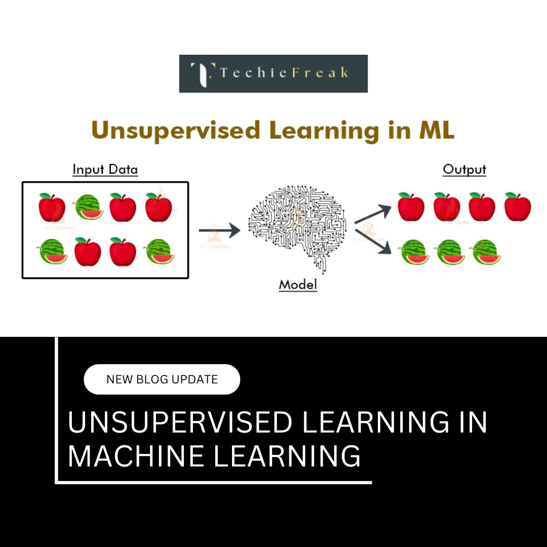
Agglomerative Hierarchical Clustering (AHC) is a bottom-up approach where each data point starts as its own cluster, and pairs of clusters are merged as we move up the hierarchy. The main goal of hierarchical clustering is to create a tree-like structure called a dendrogram, which shows how clusters are merged or split at each step.

Steps to Implement Agglomerative Hierarchical Clustering:

1. Import Necessary Libraries
2. Prepare the Data
3. Compute Distance Matrix
4. Choose Linkage Method
5. Perform Clustering using Agglomerative Clustering
6. Plot the Dendrogram
7. Determine the Optimal Number of Clusters

Step-by-Step Implementation:

Step 1: Import Necessary Libraries

We'll start by importing the necessary libraries: numpy, pandas, scikit-learn for model building, and matplotlib for visualization.

import numpy as np
import pandas as pd
import matplotlib.pyplot as plt
from sklearn.cluster import AgglomerativeClustering
from scipy.cluster.hierarchy import dendrogram, linkage

• AgglomerativeClustering: A module from sklearn to perform hierarchical clustering.
• linkage: A function from scipy that computes the hierarchical clustering linkage matrix.
• dendrogram: A function to plot the hierarchical tree (dendrogram).

Step 2: Prepare the Data

In this step we will read the data from some of the open repositories like Kaggle dataset, UCI Machine Learning Repository etc and explore the data to understand the features and its importance.

Here, we'll generate some random data or use an example dataset to demonstrate the clustering.

# Example dataset
from sklearn.datasets import make_blobs

# Generating random dataset
X, y = make_blobs(n_samples=10, centers=3, random_state=42)
print("Input Features : ")
print(X[:5])

print("Target:  ")  
print(y[:5])

Output:
Input Features : 
[[-5.41397842 -7.10588589]
 [-7.42400992 -6.769187  ]
 [ 3.62704772  2.28741702]
 [-6.81209899 -8.30485778]
 [-2.26723535  7.10100588]]
Target:  
[2 2 1 2 0]

This will create a dataset X with 10 samples and 3 centers (clusters).

Step 3: Compute Distance Matrix

To perform hierarchical clustering, a distance matrix is calculated to measure the distance between pairs of data points. In agglomerative clustering, this matrix is used to merge the closest clusters.

# Computing the linkage matrix using 'ward' method (other methods: 'single', 'complete', 'average')
Z = linkage(X, method='ward')

print(Z)

Output:
[[ 5.          9.          1.00830799  2.        ]
 [ 2.          7.          1.12932761  2.        ]
 [ 8.         11.          1.57989777  3.        ]
 [ 1.          3.          1.65309398  2.        ]
 [ 0.         13.          2.02969745  3.        ]
 [ 4.         10.          2.3974868   3.        ]
 [ 6.         15.          2.7868333   4.        ]
 [12.         16.         17.20267882  7.        ]
 [14.         17.         29.98254925 10.        ]]

• Linkage Methods: The ward method minimizes the variance of clusters being merged. Other methods include 'single', 'complete', and 'average', which differ in how they compute the distance between clusters.

Step 4: Choose Linkage Method

There are several ways to compute the distance between clusters in hierarchical clustering. Common methods are:

• Ward’s method: Minimizes the variance within each cluster.
• Single linkage: The shortest distance between points in each cluster.
• Complete linkage: The maximum distance between points in each cluster.
• Average linkage: The average distance between points in each cluster.

In the previous step, we used the 'ward' method.

Step 5: Perform Clustering using AgglomerativeClustering

We now perform agglomerative clustering with the number of clusters set to 3.

# Agglomerative Clustering
model = AgglomerativeClustering(n_clusters=3, metric='euclidean', linkage='ward')
y_pred = model.fit_predict(X)

print(y_pred)

OUTPUT:
[1 1 2 1 0 0 0 2 2 0]

• n_clusters=3: Defines the number of clusters.
• metric='euclidean': Defines the distance metric (Euclidean distance is commonly used).
• linkage='ward': Specifies the linkage method.

Step 6: Plot the Dendrogram

A dendrogram provides a visual representation of the hierarchical merging of clusters.

# Plotting the Dendrogram
plt.figure(figsize=(10, 7))
dendrogram(Z)
plt.title("Dendrogram")
plt.xlabel("Data Points")
plt.ylabel("Euclidean Distance")
plt.show()

• This plot shows the hierarchical structure of the clusters. The y-axis represents the distance between merged clusters, and the x-axis shows the individual data points.

OUTPUT:

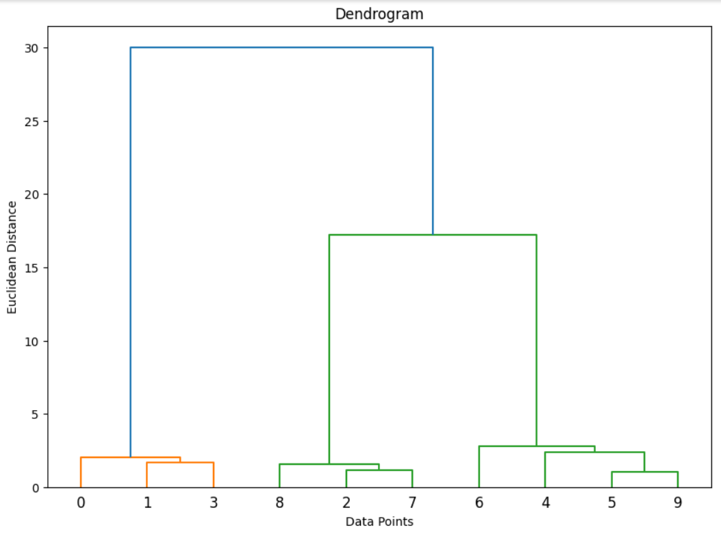
Step 7: Determine the Optimal Number of Clusters

From the dendrogram, we can choose the number of clusters by cutting the tree at a certain level. The ideal cut would show a large gap between merged clusters, indicating distinct groups.

Alternatively, if the number of clusters is known beforehand, you can specify that during the clustering step (n_clusters=3 in this example).

Final Code:

import numpy as np
import matplotlib.pyplot as plt
from sklearn.datasets import make_blobs
from sklearn.cluster import AgglomerativeClustering
from scipy.cluster.hierarchy import dendrogram, linkage

# Step 1: Generate data
X, y = make_blobs(n_samples=10, centers=3, random_state=42)

# Step 2: Perform hierarchical clustering
Z = linkage(X, method='ward')

# Step 3: Plot the dendrogram
plt.figure(figsize=(10, 7))
dendrogram(Z)
plt.title("Dendrogram")
plt.xlabel("Data Points")
plt.ylabel("Euclidean Distance")
plt.show()

# Step 4: Perform agglomerative clustering and get cluster labels
model = AgglomerativeClustering(n_clusters=3, affinity='euclidean', linkage='ward')
y_pred = model.fit_predict(X)

print("Cluster labels:", y_pred)

Conclusion:

In this implementation, we used Agglomerative Hierarchical Clustering to group the data into three clusters and visualize the hierarchical structure using a dendrogram. This method does not require the number of clusters to be specified initially but allows for visual inspection of the clustering process. However, choosing the optimal number of clusters is often subjective and may require additional methods like the elbow method or silhouette analysis.
 

Next Blog- Python implementation of Divisive Hierarchical Clustering