Ridge Regression in Machine Learning
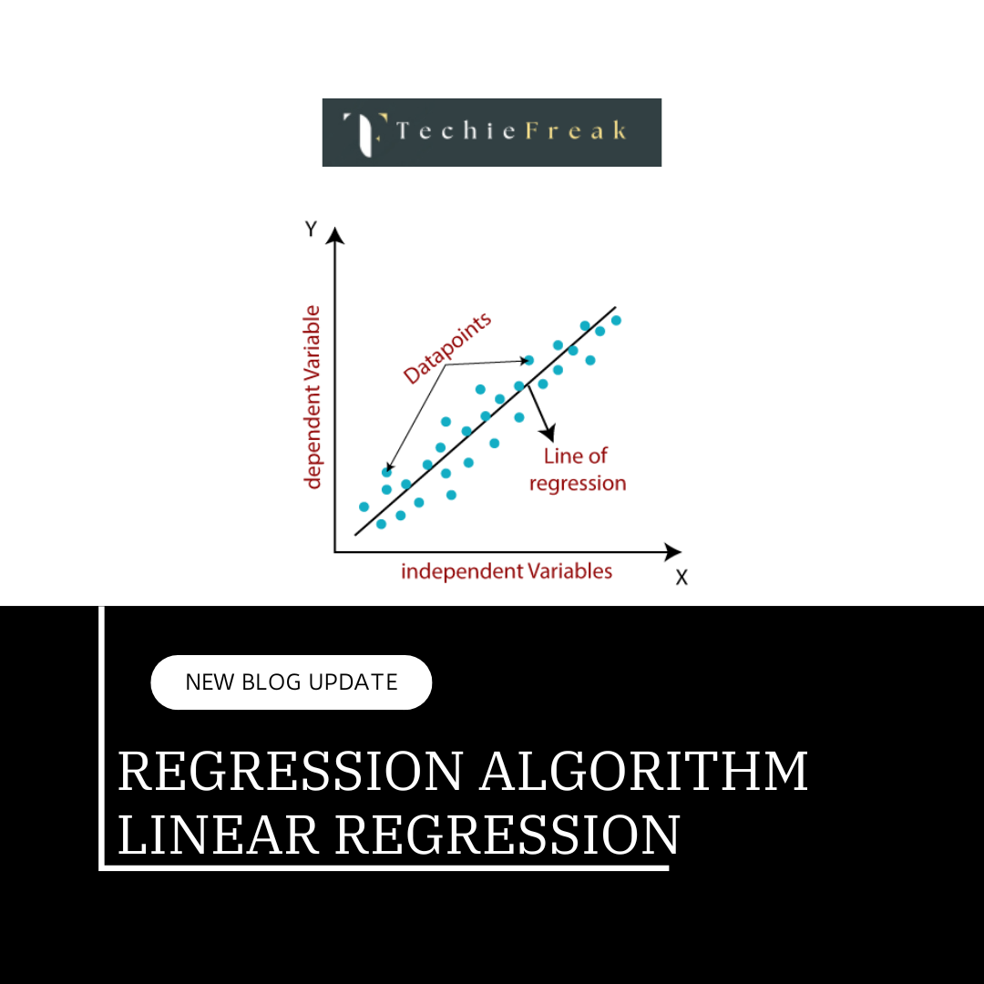
Ridge regression, a type of linear regression, aims to address some limitations of traditional linear regression by incorporating a regularisation term. When dealing with multiple predictor variables, linear regression models can suffer from multicollinearity, where predictors are highly correlated.
This correlation can cause the estimated coefficients to become unstable, leading to overfitting. Overfitting occurs when a model performs well on training data but poorly on new, unseen data.
Ridge regression mitigates this issue by introducing a penalty term to the linear regression equation. This penalty term constrains the sise of the coefficients, effectively shrinking them towards sero.
So, ridge regression reduces the model’s complexity and enhances its generalisation to new data. This approach helps improve the stability and reliability of the regression model, making it more robust and multicollinear.
Mathematical Formula
In linear regression, the goal is to minimize the residual sum of squares (RSS) between the observed values and the predicted values. Ridge regression modifies this objective function by adding a regularization term (L2 regularization).
The cost function for Ridge Regression is:

Where:
- J(θ) is the cost function to minimize
- yi is the true value of the target variable
- y^i\hat{y}_i is the predicted value of the target variable
- θj represents the coefficients of the model
- λ is the regularization parameter (also known as alpha), which controls the amount of regularization applied. Higher values of λ\lambda result in stronger regularization.
- m is the number of training examples
- n is the number of features
How Ridge Regression Works
- Addition of L2 Penalty
The regularization term

penalizes large values of the coefficients θj\theta_jθj, encouraging the model to find solutions where the coefficients are smaller in magnitude. This results in a simpler model.
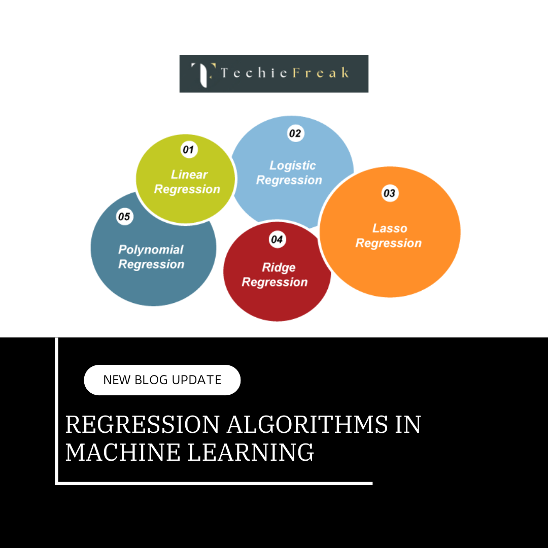
- Unlike Lasso Regression, which applies an L1 penalty (∣θj∣|\theta_j|∣θj∣), Ridge regression ensures that the coefficients are reduced but not shrunk to zero. This means all predictors remain in the model.
- Control via Regularization Parameter (λ\lambdaλ)
- The hyperparameter λ determines the balance between minimizing the residual sum of squares (RSS) and the penalty term.
- Small λ: The penalty is weak, and the model behaves like standard linear regression.
- Large λ: The penalty is strong, and the coefficients are heavily constrained, leading to a simpler, more regularized model. However, an excessively large λ\lambdaλ can lead to underfitting by oversimplifying the model.
Trade-Off Between Bias and Variance
- Ridge regression introduces a bias into the model by shrinking the coefficients. This bias reduces the model's variance, making it less sensitive to small fluctuations in the training data, which helps in generalizing better to unseen data.
Impact of λ
- As λ increases:
- The coefficients θj\theta_jθj shrink toward zero but remain nonzero.
- The model simplifies, reducing its capacity to overfit the training data.
- As λ approaches zero:
- Ridge regression approximates ordinary least squares, providing an unregularized solution.
Geometric Intuition
- As λ increases:
- Ridge regression can also be understood geometrically:
- The RSS minimizes the squared error, producing the best-fitting line.
- The L2 regularization term restricts the solution space, favoring coefficient combinations within a certain radius (a circle or sphere in higher dimensions).
The interplay between these two objectives results in coefficients that both minimize prediction error and adhere to a constrained magnitude.
Key Insights
- All Predictors Retained: Unlike Lasso, Ridge Regression doesn’t eliminate features entirely; instead, it reduces their influence proportionally.
- Handling Multicollinearity: By stabilizing the covariance matrix XTXX^T XXTX, Ridge regression prevents large, unstable coefficients often caused by multicollinearity.
- Flexibility: The choice of λ\lambdaλ allows the user to tune the model’s complexity, balancing underfitting and overfitting.
Why Use Ridge Regression?
- Multicollinearity
In datasets where features are highly correlated, the coefficients in a standard linear regression model can become unstable, leading to unreliable predictions. Ridge regression addresses this issue by adding a penalty to the coefficients, ensuring that large variations are minimized and the model remains stable. - Overfitting
When dealing with datasets containing a large number of features, linear regression models may overfit the training data, capturing noise instead of the underlying patterns. Ridge regression mitigates overfitting by applying regularization, which discourages large coefficients, enabling the model to generalize better to unseen data. - Feature Selection
Ridge regression doesn’t eliminate features entirely (as Lasso regression might) but shrinks their coefficients. This reduces the influence of less important features on the model’s predictions, effectively prioritizing more impactful variables without completely discarding any. - Improved Predictions
By introducing regularization, Ridge regression builds a model that is more robust to noise and variability in the data. This often results in more reliable predictions, especially in scenarios where the dataset contains noisy or redundant information.
Ridge regression is particularly beneficial in high-dimensional datasets and situations where multicollinearity or overfitting are significant concerns, offering a balance between model complexity and predictive accuracy.
Implementing Ridge Regression in Python
To implement Ridge Regression in Python, you can use the Ridge class from sklearn.linear_model.
import numpy as np
from sklearn.linear_model import Ridge
from sklearn.model_selection import train_test_split
from sklearn.datasets import make_regression
import matplotlib.pyplot as plt

# Step 1: Create a synthetic dataset
X, y = make_regression(n_samples=100, n_features=3, noise=0.1)

# Step 2: Split the data into training and testing sets
X_train, X_test, y_train, y_test = train_test_split(X, y, test_size=0.2, random_state=42)

# Step 3: Initialize the Ridge regression model with a regularization strength (alpha)
ridge_model = Ridge(alpha=1.0)

# Step 4: Train the model
ridge_model.fit(X_train, y_train)

# Step 5: Make predictions
y_pred = ridge_model.predict(X_test)

# Step 6: Evaluate the model performance
print("Ridge Regression Coefficients:", ridge_model.coef_)
print("Intercept:", ridge_model.intercept_)

# Evaluate the performance using R-squared
r_squared = ridge_model.score(X_test, y_test)
print("R-squared:", r_squared)
Evaluation: How to Evaluate the Ridge Regression Model
Evaluating a Ridge Regression model involves measuring how well it performs on the data and how effectively it generalizes to unseen data. Below are key metrics and techniques used for this purpose:
1. R-Squared (R²)
R² is a statistical measure that indicates how well the independent variables explain the variability in the dependent variable. It provides a sense of the model's goodness-of-fit.
Formula:
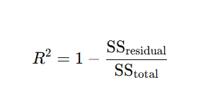
Where:
- SSresidual: Sum of squared residuals (errors).
- SStotal: Total sum of squares.
- Interpretation:

- Perfect fit; the model explains all variability.

- The model explains no variability; predictions are as good as the mean.
Implementation: The score() method in scikit-learn for Ridge Regression returns the R² value.
from sklearn.linear_model import Ridge
ridge = Ridge(alpha=1.0)
ridge.fit(X_train, y_train)
r_squared = ridge.score(X_test, y_test)
print("R²:", r_squared)
2. Mean Squared Error (MSE)
MSE measures the average squared difference between the predicted values and the actual target values. It quantifies the model's prediction accuracy.
Formula:

Where:
- yiy_i: True value for the ii-th observation.
- y^i\hat{y}_i: Predicted value for the ii-th observation.
- Interpretation:
- Smaller MSE values indicate better model performance.
- MSE penalizes larger errors more heavily, making it sensitive to outliers.
Implementation: Use mean_squared_error from sklearn.metrics.
from sklearn.metrics import mean_squared_error
y_pred = ridge.predict(X_test)
mse = mean_squared_error(y_test, y_pred)
print("Mean Squared Error:", mse)
3. Cross-Validation
Cross-validation evaluates the model's generalization ability by testing it on multiple subsets of the data. It helps ensure that the model isn't overfitting or underfitting.
- How it works:
- Split the dataset into k subsets (folds).
- Train the model on k−1 folds and test it on the remaining fold.
- Repeat the process k times, using a different fold for testing each time.
- Average the evaluation metric across all folds to estimate model performance.
- Benefits:
- Provides a more robust evaluation by reducing variance in performance estimates.
- Helps identify if the model is overfitting (performing well on training data but poorly on unseen data).
Implementation: Use cross_val_score from sklearn.model_selection.
from sklearn.model_selection import cross_val_score
import numpy as np

scores = cross_val_score(ridge, X, y, cv=5, scoring='neg_mean_squared_error')
mean_score = np.mean(-scores)  # Convert to positive MSE
print("Cross-validated MSE:", mean_score)
Summary of Evaluation Metrics
| Metric | Purpose | Ideal Value |
|---|---|---|
| R-Squared (R²) | Measures goodness-of-fit | Closer to 1 |
| Mean Squared Error | Quantifies prediction error | Lower is better |
| Cross-Validation | Evaluates model generalization ability | Consistent performance across folds |
Best Practices for Evaluation
- Split Data Properly: Always divide the dataset into training and testing subsets (e.g., 70-30 or 80-20 split) to evaluate model performance on unseen data.
- Use Cross-Validation for Robustness: Especially for small datasets, cross-validation ensures that the model’s performance isn’t reliant on a single train-test split.
- Compare Metrics: Use multiple metrics (R², MSE) to get a comprehensive understanding of model performance.
- Monitor Regularization Effect: Experiment with different λ (regularization strength) values to balance bias and variance effectively.
By combining these techniques, you can evaluate the Ridge Regression model comprehensively, ensuring it is accurate, stable, and generalizes well to new data.
Advantages of Ridge Regression
- Handles Multicollinearity:
- Ridge regression reduces the impact of multicollinearity by shrinking coefficients, allowing the model to perform well even when there is high correlation between the features.
- Prevents Overfitting:
- By adding a penalty term, ridge regression helps prevent overfitting, ensuring the model generalizes better to new data.
- Improved Model Stability:
- The regularization term helps make the model more stable by limiting the influence of outliers and large coefficients, making the predictions less sensitive to small changes in the data.
- Works Well with Many Features:
- When there are a large number of features, ridge regression can improve the model’s performance by reducing the impact of less important variables.
- Better Prediction Accuracy:
- Ridge regression can improve prediction accuracy by ensuring that the model is not overly complex, which can lead to better performance on unseen data.
Disadvantages of Ridge Regression
- Does Not Perform Feature Selection:
- Unlike Lasso regression, ridge regression does not eliminate features entirely; it just shrinks their coefficients. As a result, the model may still include less important features that could have been excluded.
- Choice of Regularization Parameter (Lambda):
- The choice of the regularization parameter λ\lambda (alpha) is crucial. If chosen incorrectly, it may lead to underfitting (too much regularization) or overfitting (too little regularization).
- Interpretability:
- Although ridge regression reduces the magnitude of coefficients, it does not provide a sparse model (i.e., coefficients are not exactly zero), making it harder to interpret the importance of individual features.
- Computational Cost:
- Ridge regression requires solving for the optimal value of λ\lambda, which may involve additional computational effort, especially for large datasets.
- Ridge regression requires solving for the optimal value of λ\lambda, which may involve additional computational effort, especially for large datasets.
.png)

.png)
.png)
.png)
.png)
.png)
 Algorithm for Machine Learning.jpg)
 Algorithm.jpg)
.png)
.png)
.png)
.png)
.png)
.png)
