Python Implementation of K-NN Algorithm

We’ll use the Iris dataset as an example for a classification task. Follow the steps below:

Step 1: Import Required Libraries

We'll start by importing the necessary libraries: numpy, pandas, scikit-learn for model building, and matplotlib for visualization.

import numpy as np
import pandas as pd
import matplotlib.pyplot as plt
from sklearn.datasets import load_iris
from sklearn.model_selection import train_test_split
from sklearn.preprocessing import StandardScaler
from sklearn.neighbors import KNeighborsClassifier
from sklearn.metrics import confusion_matrix, classification_report, accuracy_score

Step 2: Load and Explore the Dataset

In this step we will read the data from some of the open repositories like Kaggle dataset, UCI Machine Learning Repository etc and explore the data to understand the features and its importance. In this we are using Iris dataset.

# Load Iris dataset
iris = load_iris()
X = iris.data[:, :2]  # Features
y = iris.target  # Target

# Display the first few rows of data
print("Features: \n", X[:5])
print("Target: \n", y[:5])

OUTPUT:

Input Features: 
 [[5.1 3.5]
 [4.9 3. ]
 [4.7 3.2]
 [4.6 3.1]
 [5.  3.6]]

Target: 
 [0 0 0 0 0]

Step 3: Data Preprocessing

Before building the model, we need to pre-process the data. In this pre processing step, we focus on following steps:

• Missing Value Imputation, here we just remove the missing value if any feature has buy its median or Mode.
• Drop the columns which is not impacting the target
• Visualize the relationship between the feature to check if they are highly corelated to each other.
• Check if there is any categorical feature, remove it to numerical feature by applying OHE (One Hot Encoding).

 Finally, After completing all the above steps, we are in the position to split the dataset into training and testing sets using 70-30 rule (70% data will be used for training the model and 30% data will be used for testing the model) and also bring all the features in the same scale using methods like : MinMaxScaler, StandardScaler etc.

# Split the dataset into training and test sets
X_train, X_test, y_train, y_test = train_test_split(X, y, test_size=0.3, random_state=42)# Standardizing the features

scaler = StandardScaler()
X_train = scaler.fit_transform(X_train)
X_test = scaler.transform(X_test)

# Display the shape of the training and testing data
print(f"Training data shape: {X_train.shape}")
print(f"Testing data shape: {X_test.shape}")

OUTPUT:
Training data shape: (105, 2)
Testing data shape: (45, 2)

Step 4: Build and Train the K-NN Classifier Model

Now, we will create a K-NN Classifier model and train it using the training data. 

# Define the model with K=5
knn = KNeighborsClassifier(n_neighbors=5, metric='euclidean')
knn.fit(X_train, y_train)

Step 5: Validation of the model

Once the model is trained, we can make predictions on the test set.

# Predict the test results
y_pred = knn.predict(X_test)

# Display the predicted labels
print("Predicted labels: ", y_pred)

OUTPUT:
Predicted labels:  [1 0 2 1 1 0 1 2 1 1 2 0 0 0 0 1 2 1 1 2 0 2 0 2 2 2 2 2 0 0 0 0 1 0 0 2 1
 0 0 0 2 1 1 0 0]

Step 6: Evaluate the Model

After making predictions, we can evaluate the model by calculating the accuracy, confusion matrix, and classification report.

# Confusion Matrix and Accuracy
conf_matrix = confusion_matrix(y_test, y_pred)
print("Confusion Matrix:\n", conf_matrix)

# Accuracy Score
accuracy = accuracy_score(y_test, y_pred)
print("Accuracy: {:.2f}%".format(accuracy * 100))

# Classification Report
print("Classification Report:\n", classification_report(y_test, y_pred))

OUTPUT:

Confusion Matrix:
 [[19  0  0]
 [ 0 13  0]
 [ 0  0 13]]
Accuracy: 100.00%
Classification Report:
               precision    recall  f1-score   support

           0       1.00      1.00      1.00        19
           1       1.00      1.00      1.00        13
           2       1.00      1.00      1.00        13

    accuracy                           1.00        45
   macro avg       1.00      1.00      1.00        45
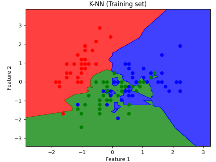
weighted avg       1.00      1.00      1.00        45

Step 7. Visualize the Results

For simplicity, visualize using two features of the Iris dataset (e.g., sepal length and width):

# Visualizing the training set
from matplotlib.colors import ListedColormap

X_set, y_set = X_train[:, :2], y_train
X1, X2 = np.meshgrid(
    np.arange(X_set[:, 0].min() - 1, X_set[:, 0].max() + 1, 0.01),
    np.arange(y_set[:, 1].min() - 1, y_set[:, 1].max() + 1, 0.01)
)

plt.contourf(X1, X2, knn.predict(np.c_[X1.ravel(), X2.ravel()]).reshape(X1.shape),
             alpha=0.75, cmap=ListedColormap(('red', 'green', 'blue')))
plt.scatter(X_set[:, 0], X_set[:, 1], c=y_set, cmap=ListedColormap(('red', 'green', 'blue')))
plt.title('K-NN (Training set)')
plt.xlabel('Feature 1')
plt.ylabel('Feature 2')
plt.show()

OUTPUT:

Outputs Explained

1. Confusion Matrix:
   • Shows how many data points were correctly and incorrectly classified.
   • Diagonal elements represent correct classifications.
2. Accuracy:
   • Measures the percentage of correctly predicted labels.
3. Visualization:
   • Decision boundaries show classification regions based on neighbors.

Next Blog- Support Vector Machine (SVM) Algorithm