Python Implementation of Logistic Regression – Step-by-Step Guide

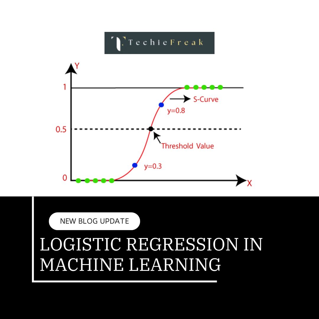
Logistic Regression is a statistical model commonly used for binary classification tasks. Despite its name, it's a linear model for binary classification, which makes it suitable for predicting the probability of an event based on given input features. Logistic Regression uses the sigmoid function to output probabilities between 0 and 1.

In this step-by-step guide, we'll implement Logistic Regression using Python and scikit-learn. We'll go through each step, from loading data to model evaluation.

1. Introduction to Logistic Regression

Logistic Regression is used for binary classification tasks (i.e., predicting one of two possible outcomes). It predicts the probability that a given input point belongs to a certain class. The sigmoid function transforms the output into a probability between 0 and 1.

The logistic function (sigmoid) is defined as:

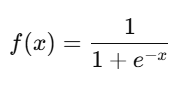
Where:

• x is the linear combination of input features.
• e is Euler's number.

2. Step-by-Step Logistic Regression Implementation

Step 1: Import Required Libraries

We'll start by importing the necessary libraries: numpy, pandas, scikit-learn for model building, and matplotlib for visualization.

#Import required libraries

import numpy as np
import pandas as pd
import matplotlib.pyplot as plt
from sklearn.model_selection import train_test_split
from sklearn.linear_model import LogisticRegression
from sklearn.metrics import accuracy_score, classification_report, confusion_matrix

Step 2: Load and Explore the Dataset

In this step we will read the data from some of the open repositories like Kaggle dataset, UCI Machine Learning Repository etc and explore the data to understand the features and its importance.

We will use a simple binary classification dataset for this example, such as the Iris dataset, but we will focus on just two classes to make it binary.

# Load the Iris dataset
from sklearn import datasets
iris = datasets.load_iris()

# Get features and target variables
X = iris.data[:, :2]  # Only take the first two features for simplicity
y = iris.target

# Convert it to a binary classification problem by taking only two classes (setosa and versicolor)
X = X[y != 2]  # Remove class 2 (virginica)
y = y[y != 2]  # Keep only classes 0 (setosa) and 1 (versicolor)

# Display the first few rows of data
print("Features: \n", X[:5])
print("Target: \n", y[:5])

Output:

Input Features: 
 [[5.1 3.5]
 [4.9 3. ]
 [4.7 3.2]
 [4.6 3.1]
 [5.  3.6]]

Target: 
 [0 0 0 0 0]

Step 3: Data Preprocessing

Before building the model, we need to pre-process the data. In this pre processing step, we focus on following steps:

• Missing Value Imputation, here we just remove the missing value if any feature has buy its median or Mode.
• Drop the columns which is not impacting the target
• Visualize the relationship between the feature to check if they are highly corelated to each other.
• Check if there is any categorical feature, remove it to numerical feature by applying OHE (One Hot Encoding).

 Finally, After completing all the above steps, we are in the position to split the dataset into training and testing sets using 80-20 rule (80% data will be used for training the model and 20% data will be used for testing the model)

# Split the dataset into training (80%) and testing (20%) sets
X_train, X_test, y_train, y_test = train_test_split(X, y, test_size=0.2, random_state=42)

# Display the shape of the training and testing data
print(f"Training data shape: {X_train.shape}")
print(f"Testing data shape: {X_test.shape}")

OUTPUT:
Training data shape: (80, 2)
Testing data shape: (20, 2)

Step 4: Build and Train the Logistic Regression Model

Now, we will create a logistic regression model and train it using the training data.

# Create a Logistic Regression model
log_reg = LogisticRegression()

# Train the model using the training data
log_reg.fit(X_train, y_train)

Step 5: Validation of the model

Once the model is trained, we can make predictions on the test set.

# Predict the labels for the test set
y_pred = log_reg.predict(X_test)

# Display the predicted labels
print("Predicted labels: ", y_pred)

OUTPUT:
Predicted labels:  [1 1 1 0 0 0 0 1 0 0 0 0 1 0 1 0 1 1 0 0]

Step 6: Evaluate the Model

After making predictions, we can evaluate the model by calculating the accuracy, confusion matrix, and classification report.

# Calculate the accuracy of the model
accuracy = accuracy_score(y_test, y_pred)
print(f"Accuracy: {accuracy * 100:.2f}%")

# Confusion Matrix
conf_matrix = confusion_matrix(y_test, y_pred)
print("Confusion Matrix: \n", conf_matrix)

# Classification Report
class_report = classification_report(y_test, y_pred)
print("Classification Report: \n", class_report)

Output:

Accuracy: 100.00%
Confusion Matrix: 
 [[12  0]
 [ 0  8]]
Classification Report: 
               precision    recall  f1-score   support

           0       1.00      1.00      1.00        12
           1       1.00      1.00      1.00         8

    accuracy                           1.00        20
   macro avg       1.00      1.00      1.00        20
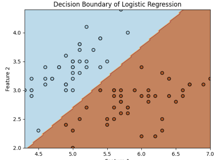
weighted avg       1.00      1.00      1.00        20

Step 7: Visualize the Decision Boundary (Optional)

To better understand how the Logistic Regression model is performing, we can plot the decision boundary.

# Plotting decision boundary
xx, yy = np.meshgrid(np.linspace(X_train[:, 0].min(), X_train[:, 0].max(), 100),
                     np.linspace(X_train[:, 1].min(), X_train[:, 1].max(), 100))

Z = log_reg.predict(np.c_[xx.ravel(), yy.ravel()])
Z = Z.reshape(xx.shape)

# Plot the data points and the decision boundary
plt.contourf(xx, yy, Z, alpha=0.75, cmap=plt.cm.Paired)
plt.scatter(X_train[:, 0], X_train[:, 1], c=y_train, edgecolors='k', cmap=plt.cm.Paired)
plt.xlabel('Feature 1')
plt.ylabel('Feature 2')
plt.title('Decision Boundary of Logistic Regression')
plt.show()

3. Conclusion

In this step-by-step guide, we successfully implemented a Logistic Regression model for a binary classification problem using Python and scikit-learn. The steps involved were:

1. Loading the dataset and preparing it for a binary classification task.
2. Preprocessing the data by splitting it into training and testing sets.
3. Training the Logistic Regression model.
4. Making predictions and evaluating the model using accuracy, confusion matrix, and classification report.
5. Visualizing the decision boundary (optional step).

Logistic Regression is an easy-to-understand and effective algorithm for binary classification tasks. You can experiment with other datasets or tune the model's hyperparameters (such as regularization strength) to improve its performance.

Next Blog- K-Nearest Neighbor(KNN) Algorithm for Machine Learning