.png)
Python Implementation of Support Vector Machine (SVM) Algorithm – Step-by-Step Guide
Support Vector Machine (SVM) is one of the most powerful and versatile machine learning algorithms, used primarily for classification tasks but also applicable to regression problems. SVM creates a hyperplane that best separates the data points into distinct classes. In this step-by-step guide, we'll walk you through the process of implementing SVM using Python, with explanations and code.
1. Introduction to SVM
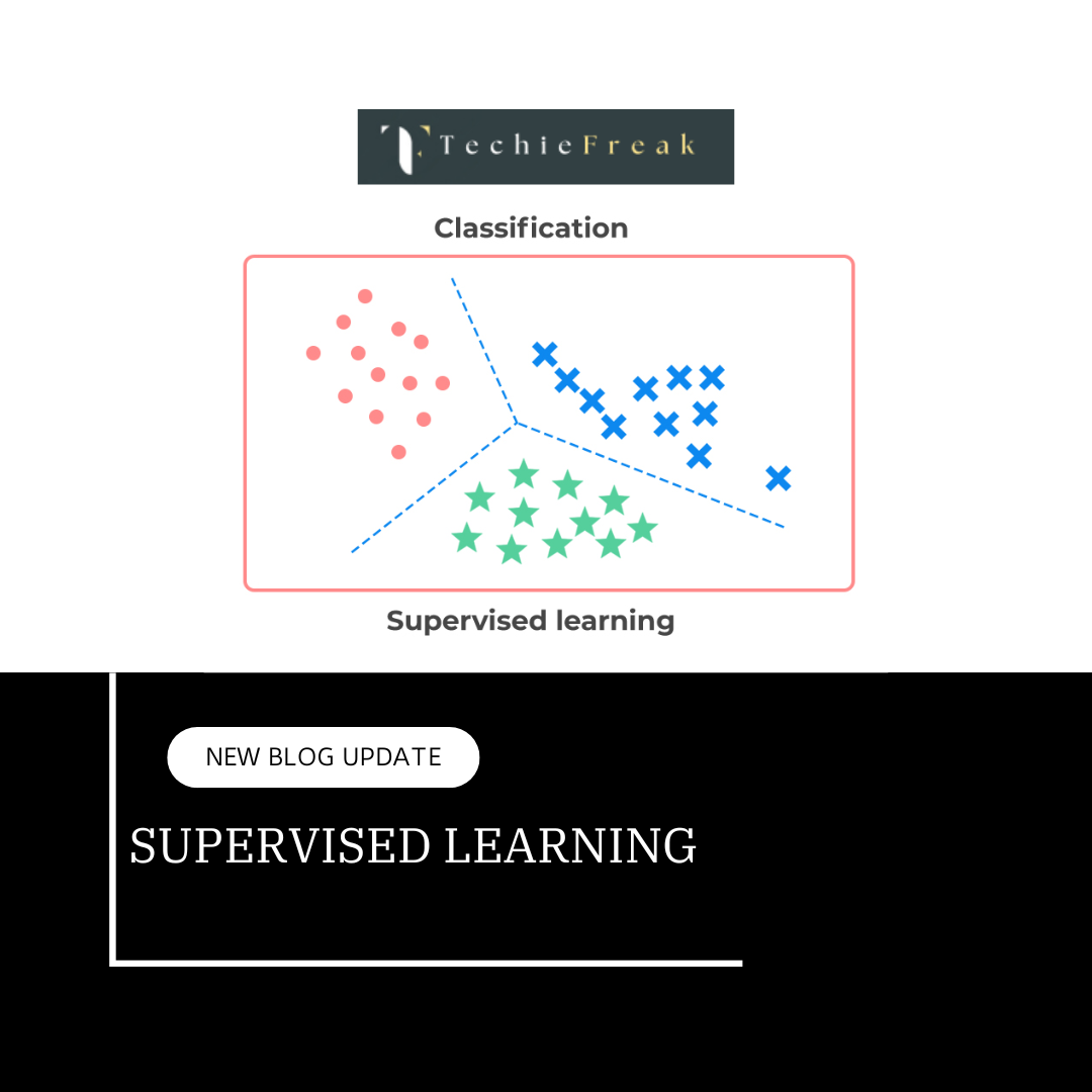
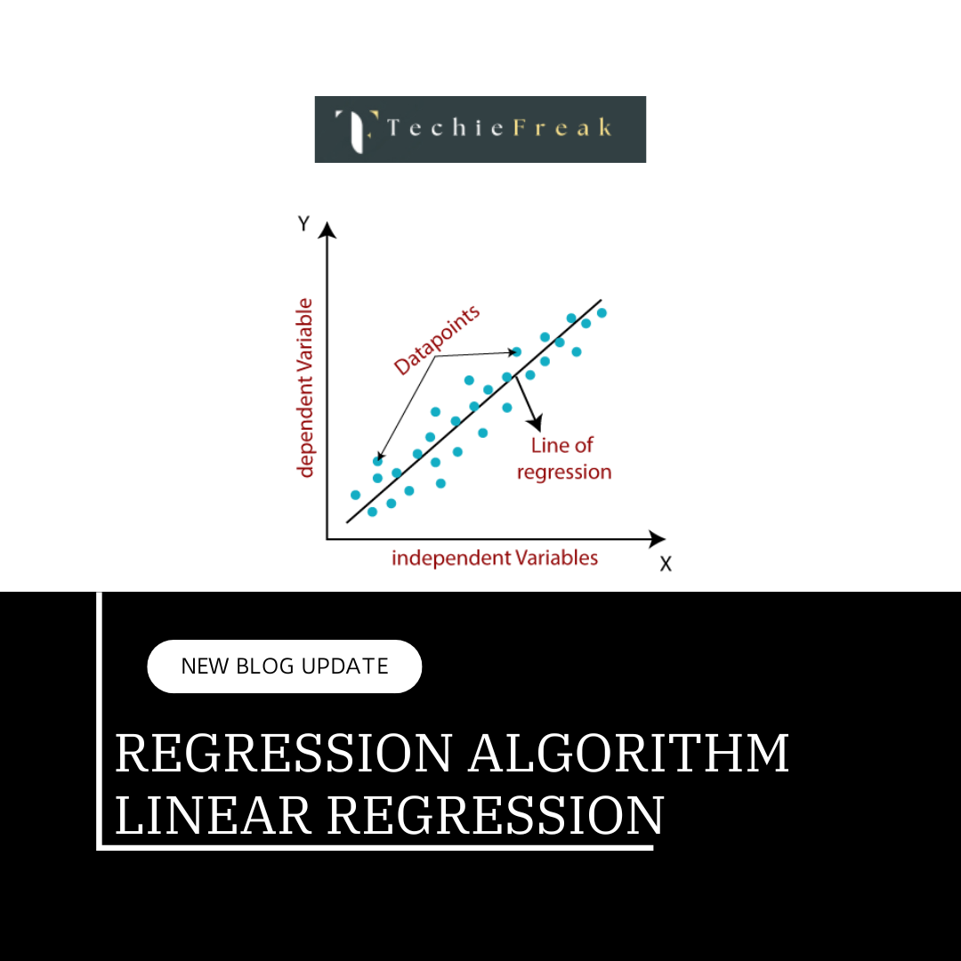
Support Vector Machine (SVM) is a supervised machine learning algorithm that can be used for both classification and regression problems. It works by finding a hyperplane that best separates the data into different classes.
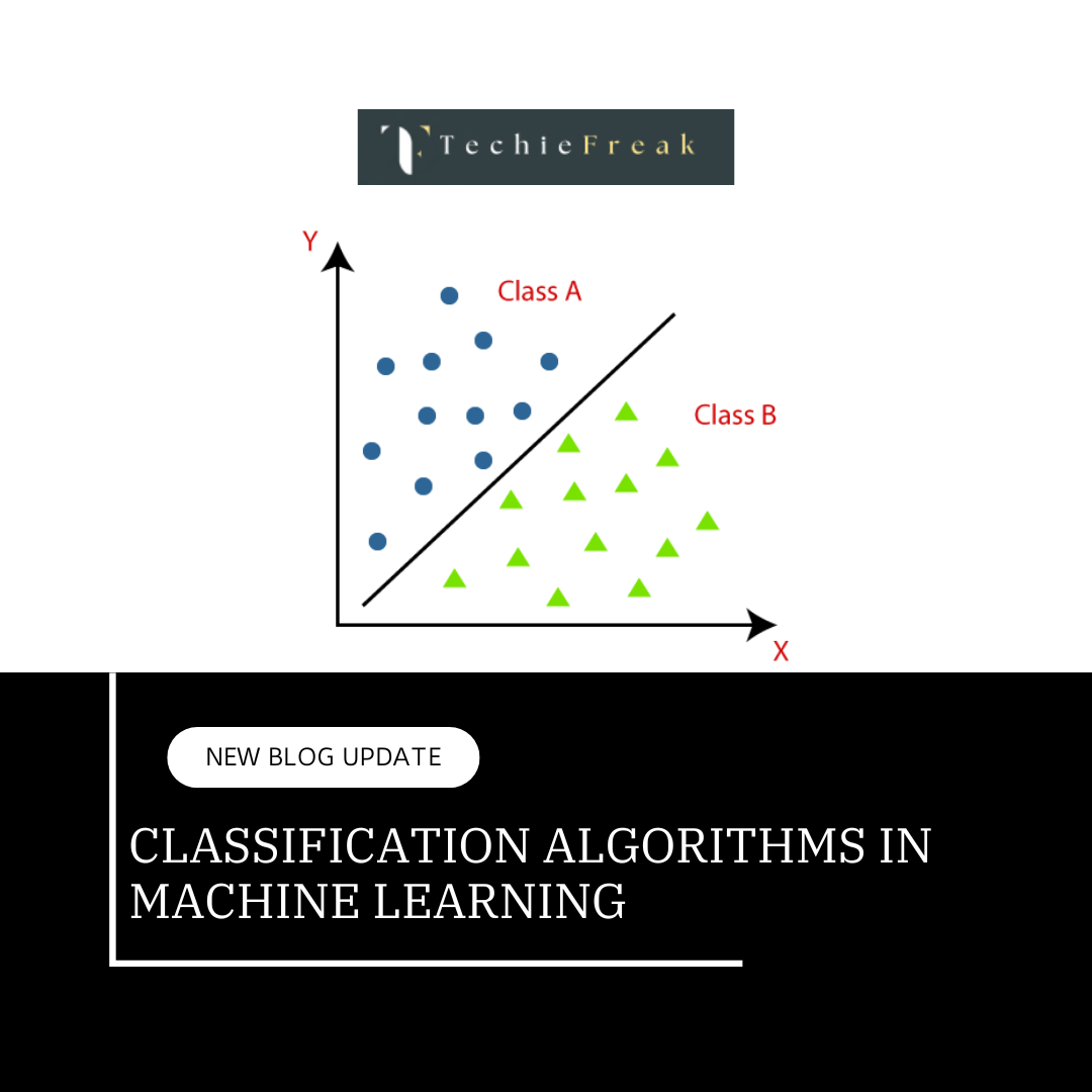
- Linear SVM: When the data is linearly separable, SVM finds the hyperplane that maximizes the margin between the classes.
- Non-linear SVM: When the data is not linearly separable, SVM uses kernels (like radial basis function (RBF), polynomial kernel) to transform the data into a higher dimension where it can be separated by a hyperplane.
2. Step-by-Step SVM Implementation
Step 1: Import Required Libraries
We'll start by importing necessary libraries. scikit-learn is the main library we will use to implement SVM, along with libraries like matplotlib for plotting graphs and pandas for handling datasets.
# Importing required libraries
import numpy as np
import matplotlib.pyplot as plt
from sklearn import datasets
from sklearn.model_selection import train_test_split
from sklearn.svm import SVC
from sklearn.metrics import accuracy_score, confusion_matrix,classification_report, accuracy_score
Step 2: Load and Explore the Dataset
In this step we will read the data from some of the open repositories like Kaggle dataset, UCI Machine Learning Repository etc and explore the data to understand the features and its importance.
For this example, we’ll use the popular Iris dataset available in scikit-learn. The Iris dataset is used to classify flowers into three species based on features such as petal length, petal width, sepal length, and sepal width.
# Load the Iris dataset
iris = datasets.load_iris()
X = iris.data  # Features
y = iris.target  # Labels (species)

# Display the first few rows of the dataset
print("Feature names:", iris.feature_names)
print("Target names:", iris.target_names)
print("First 5 rows of the data:\n", X[:5])OUTPUT:
Feature names: ['sepal length (cm)', 'sepal width (cm)', 'petal length (cm)', 'petal width (cm)']
Target names: ['setosa' 'versicolor' 'virginica']
First 5 rows of the data:
 [[5.1 3.5 1.4 0.2]
 [4.9 3.  1.4 0.2]
 [4.7 3.2 1.3 0.2]
 [4.6 3.1 1.5 0.2]
 [5.  3.6 1.4 0.2]]
Step 3: Data Preprocessing
Before building the model, we need to pre-process the data. In this pre processing step, we focus on following steps if required:
- Missing Value Imputation, here we just remove the missing value if any feature has buy its median or Mode.
- Drop the columns which is not impacting the target
- Visualize the relationship between the feature to check if they are highly corelated to each other.
- Check if there is any categorical feature, remove it to numerical feature by applying OHE (One Hot Encoding).
Finally, After completing all the above steps, we are in the position to split the dataset into training and testing sets using 80-20 rule (80% data will be used for training the model and 20% data will be used for testing the model) and also bring all the features in the same scale using methods like : MinMaxScaler, StandardScaler etc.
# Split the dataset into training and testing sets (80% train, 20% test)
X_train, X_test, y_train, y_test = train_test_split(X, y, test_size=0.2, random_state=42)

# Check the shape of the training and testing data
print("Training data shape:", X_train.shape)
print("Testing data shape:", X_test.shape)

OUTPUT:
Training data shape: (120, 4)
Testing data shape: (30, 4)
Step 4: Build and Train the SVM Model
Now that we have the training data, we can create an SVM classifier and fit it to the data. Here, we'll use a linear kernel SVM for simplicity, though we could try other kernels like RBF or polynomial also.
# Create an SVM classifier with a linear kernel
svm_model = SVC(kernel='linear')

# Train the model on the training data
svm_model.fit(X_train, y_train)

# Display the model's support vectors
print("Support Vectors:\n", svm_model.support_vectors_)

OUTPUT:
Support Vectors:
 [[4.8 3.4 1.9 0.2]
 [5.1 3.3 1.7 0.5]
 [4.5 2.3 1.3 0.3]
 [5.6 3.  4.5 1.5]
 [5.4 3.  4.5 1.5]
 [6.7 3.  5.  1.7]
 [5.9 3.2 4.8 1.8]
 [5.1 2.5 3.  1.1]
 [6.  2.7 5.1 1.6]
 [6.3 2.5 4.9 1.5]
 [6.1 2.9 4.7 1.4]
 [6.5 2.8 4.6 1.5]
 [6.9 3.1 4.9 1.5]
 [6.3 2.3 4.4 1.3]
 [6.3 2.5 5.  1.9]
 [6.3 2.8 5.1 1.5]
 [6.3 2.7 4.9 1.8]
 [6.  3.  4.8 1.8]
 [6.  2.2 5.  1.5]
 [6.2 2.8 4.8 1.8]
 [6.5 3.  5.2 2. ]
 [7.2 3.  5.8 1.6]
 [5.6 2.8 4.9 2. ]
 [5.9 3.  5.1 1.8]
 [4.9 2.5 4.5 1.7]]
Step 5: Validation of the model
Once the model is trained, we can use it to make predictions on the test data.
# Predict the class labels for the test data
y_pred = svm_model.predict(X_test)

# Display the predicted labels
print("Predicted Labels:\n", y_pred)

OUTPUT:
Predicted Labels:
 [1 0 2 1 1 0 1 2 1 1 2 0 0 0 0 1 2 1 1 2 0 2 0 2 2 2 2 2 0 0]
Step 6: Evaluate the Model
Now, let’s evaluate the performance of the model. We’ll calculate the accuracy of the model and display the confusion matrix to understand how well the model performed.
# Calculate the accuracy of the model
accuracy = accuracy_score(y_test, y_pred)
print(f"Accuracy of the SVM model: {accuracy * 100:.2f}%")

# Generate a confusion matrix
conf_matrix = confusion_matrix(y_test, y_pred)
print("Confusion Matrix:\n", conf_matrix)OUTPUT:
Accuracy of the SVM model: 100.00%
Confusion Matrix:
[[10 0 0]
[ 0 9 0]
[ 0 0 11]]
Accuracy: 100.00%
Classification Report:
precision recall f1-score support
0 1.00 1.00 1.00 10
1 1.00 1.00 1.00 9
2 1.00 1.00 1.00 11
accuracy 1.00 30
macro avg 1.00 1.00 1.00 30
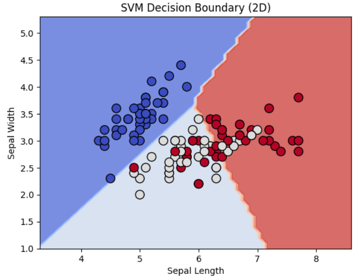
weighted avg 1.00 1.00 1.00 30Step 7: Visualizing the Results
For a better understanding of how well the SVM model is performing, we can visualize the decision boundary and the support vectors. To keep things simple, we'll use only the first two features (sepal length and sepal width) for plotting.
# Select the first two features for visualization
X_train_2D = X_train[:, :2]
X_test_2D = X_test[:, :2]

# Create and train the SVM model on the 2D data
svm_model_2D = SVC(kernel='linear')
svm_model_2D.fit(X_train_2D, y_train)

# Create a mesh grid for plotting the decision boundary
x_min, x_max = X_train_2D[:, 0].min() - 1, X_train_2D[:, 0].max() + 1
y_min, y_max = X_train_2D[:, 1].min() - 1, X_train_2D[:, 1].max() + 1
xx, yy = np.meshgrid(np.arange(x_min, x_max, 0.1),
                     np.arange(y_min, y_max, 0.1))

# Plot decision boundary
Z = svm_model_2D.predict(np.c_[xx.ravel(), yy.ravel()])
Z = Z.reshape(xx.shape)

# Plot the decision boundary and the points
plt.contourf(xx, yy, Z, alpha=0.75, cmap=plt.cm.coolwarm)
plt.scatter(X_train_2D[:, 0], X_train_2D[:, 1], c=y_train, marker='o', s=100, edgecolors='k', cmap=plt.cm.coolwarm)
plt.title("SVM Decision Boundary (2D)")

plt.xlabel("Sepal Length")
plt.ylabel("Sepal Width")
plt.show()
3. Conclusion
Support Vector Machine (SVM) is a powerful and effective algorithm, especially when the data is not linearly separable. By using kernels, we can apply SVM to more complex datasets. This implementation showed how to:
- Load a dataset,
- Split the data into training and testing sets,
- Train an SVM model,
- Make predictions,
- Evaluate the model's performance, and
- Visualize the decision boundary.
SVM works best when there is a clear margin of separation between the classes, but it can still be effective with other kernels in cases of complex, non-linear data. With this foundation, you can experiment with different datasets, kernels, and hyperparameters to get the best performance for your specific machine learning problem.
Next Blog - Decision Tree in Machine Learning
.png)
.png)
.png)
.png)
.png)
.png)
 Algorithm for Machine Learning.jpg)
 Algorithm.jpg)

.png)
.png)
.png)
.png)
.png)