What is a Polynomial Regression? 

• There are some relationships that a researcher will hypothesize is curvilinear. Clearly, such types of cases will include a polynomial term.
• Inspection of residuals. If we try to fit a linear model to curved data, a scatter plot of residuals (Y-axis) on the predictor (X-axis) will have patches of many positive residuals in the middle. Hence in such a situation, it is not appropriate.
• An assumption in the usual multiple linear regression analysis is that all the independent variables are independent. In the polynomial regression model, this assumption is not satisfied.

Why Polynomial Regression?

Polynomial regression is a type of regression analysis used in statistics and machine learning when the relationship between the independent variable (input) and the dependent variable (output) is not linear. While simple linear regression models the relationship as a straight line, polynomial regression allows for more flexibility by fitting a polynomial equation to the data.

When the relationship between the variables is better represented by a curve rather than a straight line, polynomial regression can capture the non-linear patterns in the data.

How does a Polynomial Regression work?

If we observe closely then we will realize that to evolve from linear regression to polynomial regression. We are just supposed to add the higher-order terms of the dependent features in the feature space. This is sometimes also known as feature engineering but not exactly.

When the relationship is non-linear, a polynomial regression model introduces higher-degree polynomial terms.

The general form of a polynomial regression equation of degree n is:

y=β0+β1x+β2x2+…+βnxn+ϵy=β0​+β1​x+β2​x2+…+βn​xn+ϵ

where,

• y is the dependent variable.
• x is the independent variable.
• β0,β1,…,βnβ0​,β1​,…,βn​​ are the coefficients of the polynomial terms.
• n is the degree of the polynomial.
• ϵϵ represents the error term.

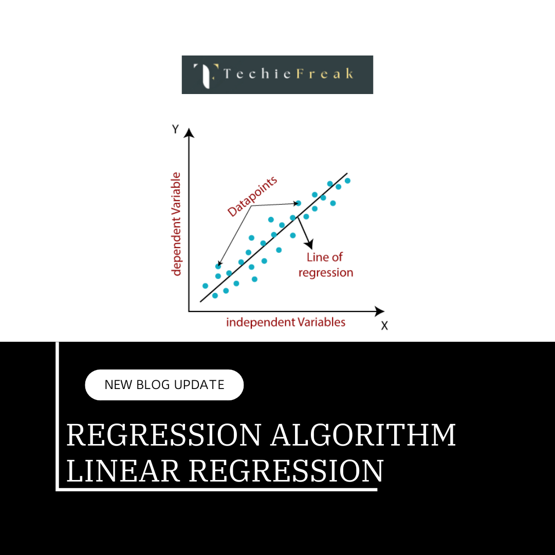
The basic goal of regression analysis is to model the expected value of a dependent variable y in terms of the value of an independent variable x. In simple linear regression, we used the following equation – 

y = a + bx + e

Here y is a dependent variable, a is the y-intercept, b is the slope and e is the error rate. In many cases, this linear model will not work out For example if we analyze the production of chemical synthesis in terms of the temperature at which the synthesis takes place in such cases we use a quadratic model.y=a+b1x+b2x2+ey=a+b1​x+b2​x2+e

Here,

• y is the dependent variable on x
• a is the y-intercept and e is the error rate.

In general, we can model it for the nth value. y=a+b1x+b2x2+….+bnxny=a+b1​x+b2​x2+….+bn​xn

Since the regression function is linear in terms of unknown variables, hence these models are linear from the point of estimation. Hence through the Least Square technique, response value (y) can be computed.

By including higher-degree terms (quadratic, cubic, etc.), the model can capture the non-linear patterns in the data.

1. The choice of the polynomial degree (n) is a crucial aspect of polynomial regression. A higher degree allows the model to fit the training data more closely, but it may also lead to overfitting, especially if the degree is too high. Therefore, the degree should be chosen based on the complexity of the underlying relationship in the data.
2. The polynomial regression model is trained to find the coefficients that minimize the difference between the predicted values and the actual values in the training data.
3. Once the model is trained, it can be used to make predictions on new, unseen data. The polynomial equation captures the non-linear patterns observed in the training data, allowing the model to generalize to non-linear relationships.

Applications of Polynomial Regression:

• Curve Fitting: When the data is expected to follow a non-linear trend but still has some relationship that can be approximated by a polynomial curve.
• Stock Market Prediction: When modeling complex price trends that are not strictly linear but exhibit curvature.
• Economics and Engineering: Polynomial regression is used in fields where relationships between variables are complex and non-linear, like in economic modeling or predicting physical phenomena.

Real-Life Example of Polynomial Regression: Predicting House Prices

In real estate, house prices often do not increase or decrease in a simple linear fashion but follow a more complex trend influenced by various factors such as the size of the house, its age, number of bedrooms, and location. A polynomial regression model can be a great tool to predict house prices based on these factors, especially when the relationship between variables is not strictly linear.

Scenario:

Let’s say you want to predict the price of a house based on its square footage (size). Initially, you might think that price increases with square footage in a linear manner, but in reality, the relationship might be curvilinear (e.g., the price may increase rapidly for larger homes, but at a diminishing rate).

Steps to Implement Polynomial Regression for House Price Prediction:

1. Data Collection: Suppose you have data for house prices (in dollars) based on their square footage (in square feet).

   Square Footage	Price (in $)
   800	180,000
   1000	200,000
   1200	230,000
   1500	300,000
   1800	350,000
   2500	500,000
   3000	550,000

2. Transform Data to Polynomial Features: We’ll use polynomial regression to predict the house price based on the square footage, taking into account that the relationship may not be linear.
3. Implementation: Here's the Python code to implement polynomial regression on this real-life data.

Code Implementation:

import numpy as np
import matplotlib.pyplot as plt
from sklearn.linear_model import LinearRegression
from sklearn.preprocessing import PolynomialFeatures

# Step 1: Define the dataset (Square Footage vs Price)
square_footage = np.array([800, 1000, 1200, 1500, 1800, 2500, 3000]).reshape(-1, 1)  # Independent variable
price = np.array([180000, 200000, 230000, 300000, 350000, 500000, 550000])  # Dependent variable (Price)

# Step 2: Transform the data to include polynomial features
poly = PolynomialFeatures(degree=3)  # Using degree 3 for a cubic relationship
square_footage_poly = poly.fit_transform(square_footage)

# Step 3: Create and train the polynomial regression model
model = LinearRegression()
model.fit(square_footage_poly, price)

# Step 4: Make predictions using the model
price_pred = model.predict(square_footage_poly)

# Step 5: Visualize the data and the polynomial regression curve
plt.scatter(square_footage, price, color='red')  # Actual data points
plt.plot(square_footage, price_pred, color='blue')  # Polynomial regression curve
plt.title('Polynomial Regression: House Prices vs Square Footage')
plt.xlabel('Square Footage')
plt.ylabel('Price (in $)')
plt.show()

# Output the model coefficients and intercept
print("Polynomial Coefficients: ", model.coef_)
print("Intercept: ", model.intercept_)

Explanation:

1. Data: The square_footage array holds the independent variable (house size in square feet), and the price array holds the dependent variable (house price).
2. Polynomial Features: The PolynomialFeatures from sklearn.preprocessing transforms the input features (square footage) into higher powers (e.g., x2x^2, x3x^3) to allow the regression model to capture non-linear patterns.
3. Linear Regression: The transformed features are then passed to LinearRegression to find the best-fit curve, which can handle polynomial relationships in the data.
4. Prediction: The trained model is used to predict house prices based on the square footage, and the results are visualized with a scatter plot (for actual data) and a line plot (for predicted prices).
5. Visualization: The plot shows how the polynomial regression curve fits the data better than a simple straight line, capturing the non-linear trend in house prices.

Output:

The polynomial regression curve will show how the price increases more rapidly for larger homes. The coefficients of the polynomial regression model will also provide insights into how different degrees of square footage (e.g., x2x^2, x3x^3) contribute to the price prediction.

Application of Polynomial Regression

The reason behind the vast use cases of the polynomial regression is that approximately all of the real-world data is non-linear in nature and hence when we fit a non-linear model on the data or a curvilinear regression line then the results that we obtain are far better than what we can achieve with the standard linear regression. Some of the use cases of the Polynomial regression are as stated below: 

• The growth rate of tissues.
• Progression of disease epidemics
• Distribution of carbon isotopes in lake sediments

Advantages & Disadvantages of using Polynomial Regression

Advantages of Polynomial Regression

1. Captures Non-Linear Relationships:
   • Polynomial regression is great for modeling non-linear relationships. When the relationship between independent and dependent variables is not linear, polynomial regression can fit curves to the data, allowing for more accurate predictions.
2. Flexible and Easy to Implement:
   • It’s relatively simple to implement, and you can easily adjust the degree of the polynomial to control the complexity of the model. With a low-degree polynomial (like quadratic or cubic), it’s easy to adapt the model to fit a wide range of data patterns.
3. Better Fit for Complex Data:
   • In cases where data shows a more complex curve (like exponential growth or diminishing returns), polynomial regression can provide a better fit than linear regression, thus improving model accuracy.
4. Generalized Approach:
   • Polynomial regression can generalize well to different types of data without needing domain-specific knowledge to identify the exact relationship. It works well for many real-world problems with unknown functional relationships.
5. Improved Predictive Performance:
   • For many datasets, polynomial regression can outperform linear regression in terms of predictive performance by fitting the curve better.

Disadvantages of Polynomial Regression

1. Overfitting:
   • One of the biggest drawbacks is that as the degree of the polynomial increases, the model may overfit the data. Overfitting occurs when the model learns the noise in the data, rather than the actual underlying pattern, making it less generalizable to new data.
2. Increased Complexity:
   • Higher-degree polynomials result in more complex models with additional parameters. This can make the model harder to interpret, especially when the degree becomes large (e.g., a 10th-degree polynomial), which may reduce its practical usability.
3. Sensitivity to Outliers:
   • Polynomial regression is highly sensitive to outliers, especially for higher-degree polynomials. A single outlier can distort the shape of the polynomial curve and affect the model's performance, leading to poor predictions.
4. Requires More Computational Power:
   • As the degree of the polynomial increases, the computational complexity also increases. This may lead to longer training times, especially with large datasets.
5. Not Always a Realistic Representation:
   • A polynomial regression curve may fit the training data well but may not always represent the underlying relationship realistically. For instance, higher-degree polynomials may result in unrealistic oscillations in the curve that don’t make sense in the context of the real-world problem.
6. Extrapolation Issues:
   • Polynomial regression may have poor performance when making predictions outside the range of the training data (extrapolation). For example, if your model is trained on a range of values from 1 to 10 and you try to predict for 100, the polynomial curve may make unreasonable predictions due to its complexity.
7. Interpretability:
   • Polynomial regression models, especially with higher degrees, can be less interpretable. For instance, determining which specific term (e.g., x2x^2, x3x^3) is responsible for a particular effect can be difficult when dealing with higher-order polynomials.

Next Topic-   Python Implementation of Polynomial Regression Model