Step 1 : Import the important Libraries
# Supress Warnings

import warnings
warnings.filterwarnings('ignore')

# Import the numpy and pandas package

import numpy as np
import pandas as pd

# Data Visualisation

import matplotlib.pyplot as plt
import seaborn as sns

from sklearn.model_selection import train_test_split
from sklearn.preprocessing import MinMaxScaler
from sklearn.linear_model import LinearRegression
from sklearn.metrics import r2_score,mean_absolute_error
Step 2 : Read an explore the data
In this step we will read the data some of the open repositories like Kaggle dataset, UCI Machine Learning Repository etc and explore the data to understand the features and its importance using the following commands:
# First download the csv file from any of the above repositories and Read the csv file
data = pd.read_csv("Housing.csv") # lets say Housing.csv file is downloaded
# show first 10 rows of the dataset
data.head(10)OUTPUT:

# show the details about dataset such as no of  rows, datatypes of each features, how many non-null values in each features.
data.info()

OUTPUT :

RangeIndex: 545 entries, 0 to 544
Data columns (total 13 columns):
 #   Column            Non-Null Count  Dtype
---  ------            --------------  -----
 0   price             545 non-null    int64
 1   area              545 non-null    int64
 2   bedrooms          545 non-null    int64
 3   bathrooms         545 non-null    int64
 4   stories           545 non-null    int64
 5   mainroad          545 non-null    object
 6   guestroom         545 non-null    object
 7   basement          545 non-null    object
 8   hotwaterheating   545 non-null    object
 9   airconditioning   545 non-null    object
 10  parking           545 non-null    int64
 11  prefarea          545 non-null    object
 12  furnishingstatus  545 non-null    object
dtypes: int64(6), object(7)
memory usage: 55.5+ KB

# Show the details about each features such as min value, max value, std, mean value etc, which helps to check the outliers in the feature at high level
data.describe()

OUTPUT :
	price	area	bedrooms	bathrooms	stories	parking
count	5.450000e+02	545.000000	545.000000	545.000000	545.000000	545.000000
mean	4.766729e+06	5150.541284	2.965138	1.286239	1.805505	0.693578
std	1.870440e+06	2170.141023	0.738064	0.502470	0.867492	0.861586
min	1.750000e+06	1650.000000	1.000000	1.000000	1.000000	0.000000
25%	3.430000e+06	3600.000000	2.000000	1.000000	1.000000	0.000000
50%	4.340000e+06	4600.000000	3.000000	1.000000	2.000000	0.000000
75%	5.740000e+06	6360.000000	3.000000	2.000000	2.000000	1.000000
max	1.330000e+07	16200.000000	6.000000	4.000000	4.000000	3.000000
Step 3 : Outlier Analysis
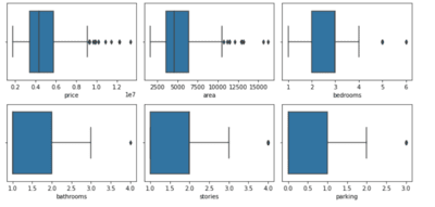
In this step we will check the outliers using the box plot
fig, axs = plt.subplots(2,3, figsize = (10,5))
plt1 = sns.boxplot(data['price'], ax = axs[0,0]).set(xlabel='price')
plt2 = sns.boxplot(data['area'], ax = axs[0,1]).set(xlabel='area')
plt3 = sns.boxplot(data['bedrooms'], ax = axs[0,2]).set(xlabel='bedrooms')
plt1 = sns.boxplot(data['bathrooms'], ax = axs[1,0]).set(xlabel='bathrooms')
plt2 = sns.boxplot(data['stories'], ax = axs[1,1]).set(xlabel='stories')
plt3 = sns.boxplot(data['parking'], ax = axs[1,2]).set(xlabel='parking')

plt.tight_layout()OUTPUT:
Step 4 : Outlier Treatment
From the previous step if we see that there is some outliers in any of the features, we will remove the outliers from those features. If we see the above image , it clearly shows that price and area have the outliers. So lets remove the outliers from them
# outlier treatment for price

Q1 = data.price.quantile(0.25) # data['price'].quantile(0.25)
Q3 = data.price.quantile(0.75)
IQR = Q3 - Q1
data = data[(data.price >= Q1 - 1.5*IQR) & (data.price <= Q3 + 1.5*IQR)]
print(Q3,Q1)

# outlier treatment for area

Q1 = data.area.quantile(0.25)
Q3 = data.area.quantile(0.75)

IQR = Q3 - Q1
data = data[(data.area >= Q1 - 1.5*IQR) & (data.area <= Q3 + 1.5*IQR)]

len(data)  # gives the length (no of rows) in the dataset
data.columns # shows name of features in the dataset
Step 5 : Correlation in the features
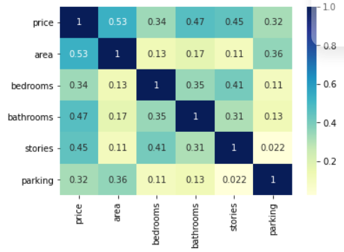
In this step we will try to see if there is any correlation between the numerical features. In heatmap the value near to 1 shows high correlation between the features and value close to zero or -ve shows low correlation.
# plotting correlation heatmap
dataplot = sns.heatmap(data[['price', 'area', 'bedrooms', 'bathrooms', 'stories','parking']].corr(), cmap="YlGnBu", annot=True)

# displaying heatmap
plt.show()OUTPUT:
Step 6 : Visualizing categorical variables
In this step let's try to analyse the categorical variable w.r.t target variable (Price) to see the relationship between them using box plot.
#Visualizing categorical variables

plt.figure(figsize=(20, 12))
plt.subplot(2,3,1)
sns.boxplot(x = 'mainroad', y = 'price', data = data)
plt.subplot(2,3,2)
sns.boxplot(x = 'guestroom', y = 'price', data = data)
plt.subplot(2,3,3)
sns.boxplot(x = 'basement', y = 'price', data = data)
plt.subplot(2,3,4)
sns.boxplot(x = 'hotwaterheating', y = 'price', data = data)
plt.subplot(2,3,5)
sns.boxplot(x = 'airconditioning', y = 'price', data = data)
plt.subplot(2,3,6)
sns.boxplot(x = 'furnishingstatus', y = 'price', data = data)OUTPUT:


Step 7 : Convert data to features
In this step we will convert the categorical data to numerical data as the computer only understands the numerical data. For this we can use the One Hot Encoding technique.
# List of variables to map

cat_features =  ['mainroad', 'guestroom', 'basement', 'hotwaterheating', 'airconditioning', 'prefarea']

# Defining the map function
def create_features(x):
    return x.map({'yes': 1, "no": 0})

# Applying the function to the housing list
data[cat_features] = data[cat_features].apply(create_features)

data.head(10)OUTPUT:

#Create dummy features for categorical variables

data_cat = pd.get_dummies(data['furnishingstatus'],drop_first=True)  # this will convert 'furnishingstatus' feature to numerical feature.

data_cat.head(10)


OUTPUT:


   semi-furnished	unfurnished
15	   1	           0
16	   0	           1
17	   0	           0
18	   0	           0
19	   1	           0
         ...	...	...
115	   1	           0
116	   0	           1
117	   0	           0
118	   0	           0
119	   1	           0
Lets concatenate the data and data_cat tables.
data = pd.concat([data, data_cat], axis = 1)
data.drop(['furnishingstatus'], axis = 1, inplace = True)
data.head(10)
Step 8 : Train test split and Data Scaling
In this step we will split the dataset into training and testing datasets and also apply the scaling to bring all the features on the same scale.
#np.random.seed(0) # not must to do
df_train, df_test = train_test_split(data, train_size = 0.8, test_size = 0.2, random_state = 100)

#creating MinMaxScaler instance
scaler = MinMaxScaler()

# Apply scaler() to all the columns except the 'yes-no' and 'dummy' variables as these variables are already in 0-1 range
num_vars = ['area', 'bedrooms', 'bathrooms', 'stories', 'parking']

df_train[num_vars] = scaler.fit_transform(df_train[num_vars])

df_train.describe()

df_test[num_vars] = scaler.transform(df_test[num_vars])

df_test.describe()

y_train = df_train.pop('price') # df_train['price'] #labels in training data
x_train = df_train # features in training data

y_test = df_test.pop('price') # df_test['price'] #lables in test data
x_test = df_test # features in test data
Step 9 : Fit the Linear Regression Model
In this step we will create the instance of the linear Regression Model and will train the model with training dataset.
# Creating the LR Model instance
lr_model = LinearRegression()
lr_model.fit(x_train, y_train) # training the model

#Let's see the summary of our linear model
print(lr_model.coef_)

OUTPUT :
[2527088.9929434   193000.69186716 1520868.29320012 1471086.25857166
  387163.28407339  107665.08808556  320841.59283444  759920.54717187
  657331.9144279   517028.53121592  627668.26091734  -27828.72692791
 -407917.30736564]

# this is for our understanding - not needed for LR model
import numpy as np
importance = np.array(lr_model.coef_)
importance = importance / sum(importance)
print(importance )

OUTPUT:
[ 0.29201677  0.02230212  0.17574333  0.16999079  0.0447385   0.0124412
  0.03707472  0.08781232  0.07595773  0.05974503  0.07252996 -0.00321574
 -0.04713672]

for z in range(len(list(x_train.columns))):
    print("The Importance coefficient for {} is {}".format(x_train.columns[z], importance[z]))

OUTPUT:
The Importance coefficient for area is 0.29201676766716095
The Importance coefficient for bedrooms is 0.022302118506294103
The Importance coefficient for bathrooms is 0.17574333324545388
The Importance coefficient for stories is 0.16999078995129616
The Importance coefficient for mainroad is 0.04473849994607111
The Importance coefficient for guestroom is 0.012441196610463412
The Importance coefficient for basement is 0.03707472318320364
The Importance coefficient for hotwaterheating is 0.08781231784422613
The Importance coefficient for airconditioning is 0.07595772902011237
The Importance coefficient for parking is 0.05974502714347178
The Importance coefficient for prefarea is 0.07252995728767934
The Importance coefficient for semi-furnished is -0.003215737517939552
The Importance coefficient for unfurnished is -0.047136722887493224

print(lr_model.intercept_) # Prints Y intercepts

OUTPUT:
2189813.38551533
Step 10 : Residual Analysis
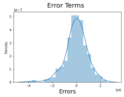
- Residual analysis is typically performed on the training data rather than the test data.
- The purpose of residual analysis is to assess the performance and
- Assumptions of your regression model during the training phase.
y_train_pred = lr_model.predict(x_train)
residuals = (y_train_pred - y_train)

# Plot the histogram of the error terms
fig = plt.figure()
sns.distplot(residuals, bins = 20)
fig.suptitle('Error Terms', fontsize = 20)                  # Plot heading
plt.xlabel('Errors', fontsize = 18) # X-labelOUTPUT:
Step 11 : Create predictions and evaluate model
# Making predictions
y_test_pred = lr_model.predict(x_test)

r2_score(y_test, y_test_pred)
mean_absolute_error(y_test, y_test_pred)

# Plotting y_test and y_pred to understand the spread.
fig = plt.figure()
plt.scatter(y_test,y_test_pred)
fig.suptitle('y_test vs y_test_pred', fontsize=20)              # Plot heading
plt.xlabel('y_test', fontsize=18)                          # X-label
plt.ylabel('y_test_pred', fontsize=16)                          # Y-label
.png)
.png)
.png)
.png)
.png)
.png)
 Algorithm for Machine Learning.jpg)
 Algorithm.jpg)

.png)
.png)
.png)
.png)
.png)
.png)
