Machine Learning is a branch of Artificial intelligence that focuses on the development of algorithms and statistical models that can learn from and make predictions on data. Linear regression is also a type of machine-learning algorithm more specifically a supervised machine-learning algorithm that learns from the labelled datasets and maps the data points to the most optimized linear functions, which can be used for prediction on new datasets.
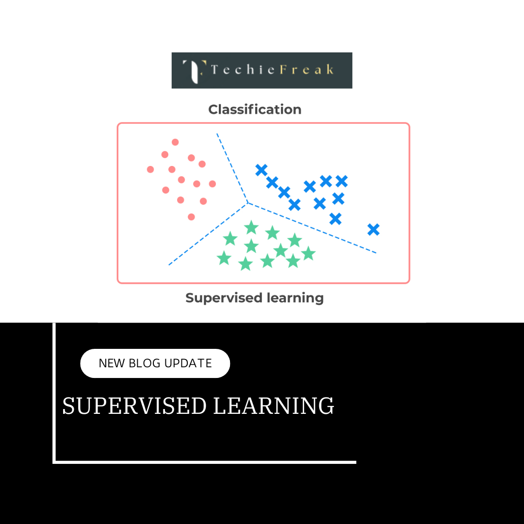
First off we should know what supervised machine learning algorithms is. It is a type of machine learning where the algorithm learns from labelled data. Labeled data means the dataset whose respective target value is already known. Supervised learning has two types:
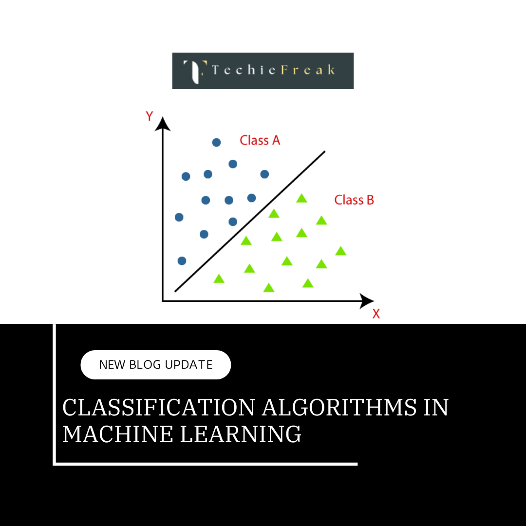
- Classification: It predicts the class of the dataset based on the independent input variable. Class is the categorical or discrete values. like the image of an animal is a cat or dog?
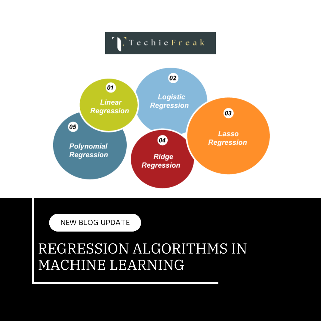
- Regression: It predicts the continuous output variables based on the independent input variable. like the prediction of house prices based on different parameters like house age, distance from the main road, location, area, etc.
Here, we will discuss one of the simplest types of regression i.e. Linear Regression.
Why is Linear Regression Important?
- Interpretability: Coefficients offer insights into variable relationships.
- Simplicity: Easy to implement and foundational for advanced techniques.
- Versatility: Forms the basis for regularization techniques, support vector machines, and more.
Types of Linear Regression
There are two main types of linear regression:
Simple Linear Regression
This is the simplest form of linear regression, and it involves only one independent variable and one dependent variable. The equation for simple linear regression is:
y=β0+β1X
where:
- Y is the dependent variable
- X is the independent variable
- β0 is the intercept
- β1 is the slope
Multiple Linear Regression
This involves more than one independent variable and one dependent variable. The equation for multiple linear regression is:
y=β0+β1X1+β2X2+………βnXny=β0+β1X1+β2X2+………βnXn
where:
- Y is the dependent variable
- X1, X2, …, Xn are the independent variables
- β0 is the intercept
- β1, β2, …, βn are the slopes
The algorithm aims to find the best Fit Line equation that can predict the values based on the independent variables.
In regression set of records are present with X and Y values and these values are used to learn a function so if you want to predict Y from an unknown X this learned function can be used. In regression we have to find the value of Y, So, a function is required that predicts continuous Y in the case of regression given X as independent features.
What is the best Fit Line?
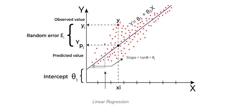
In linear regression, the primary goal is to identify the best-fit line, which minimizes the error between the predicted values and the actual values. The best-fit line ensures that the error is as small as possible.
The equation for the best-fit line defines a straight line that explains the relationship between the independent and dependent variables. The slope of this line indicates how much the dependent variable changes with a unit increase in the independent variable(s).
Here, the dependent variable, often denoted as Y, is also called the target variable, while the independent variable, represented as X, serves as the predictor for Y. The independent variable can consist of one or multiple features describing the problem.
Linear functions are the simplest form of functions used for regression. Linear regression predicts the value of the dependent variable (Y) based on the given value of the independent variable (X). For example, if X represents work experience and Y represents salary, the regression line acts as the best-fit line for the model, illustrating the relationship between experience and salary.
To find the best-fit line, we rely on the cost function, which helps determine the optimal values for the weights or coefficients of the line. Since different values of these coefficients lead to different regression lines, the cost function ensures that the chosen values yield the line with the least error.
Hypothesis function in Linear Regression
As we have assumed earlier that our independent feature is the experience i.e X and the respective salary Y is the dependent variable. Let’s assume there is a linear relationship between X and Y then the salary can be predicted using:
Y^=θ1+θ2X
OR
y^i=θ1+θ2xi
Here,
- yiϵY(i=1,2,⋯,n) are labels to data (Supervised learning)
- xiϵX(i=1,2,⋯,n) are the input independent training data (univariate – one input variable(parameter))
- yi^ϵY^(i=1,2,⋯,n) are the predicted values.
The model gets the best regression fit line by finding the best θ1 and θ2 values.
- θ1: intercept
- θ2: coefficient of x
Once we find the best θ1 and θ2 values, we get the best-fit line. So when we are finally using our model for prediction, it will predict the value of y for the input value of x.
How to update θ1 and θ2 values to get the best-fit line?
To achieve the best-fit regression line, the model aims to predict the target value Y^ Y^ such that the error difference between the predicted value Y^ Y^ and the true value Y is minimum. So, it is very important to update the θ1 and θ2 values, to reach the best value that minimizes the error between the predicted y value (pred) and the true y value (y).

Cost function for Linear Regression
The cost function or the loss function is nothing but the error or difference between the predicted value Y^ and the true value Y.
In Linear Regression, the Mean Squared Error (MSE) cost function is employed, which calculates the average of the squared errors between the predicted values y^i and the actual values yi. The purpose is to determine the optimal values for the intercept θ1θ1 and the coefficient of the input feature θ2θ2 providing the best-fit line for the given data points. The linear equation expressing this relationship is y^i=θ1+θ2xi.
MSE function can be calculated as:

Utilizing the MSE function, the iterative process of gradient descent is applied to update the values of \θ1&θ2. This ensures that the MSE value converges to the global minima, signifying the most accurate fit of the linear regression line to the dataset.
This process involves continuously adjusting the parameters \(\theta_1\) and \(\theta_2\) based on the gradients calculated from the MSE. The final result is a linear regression line that minimizes the overall squared differences between the predicted and actual values, providing an optimal representation of the underlying relationship in the data.
Gradient Descent for Linear Regression
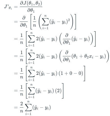
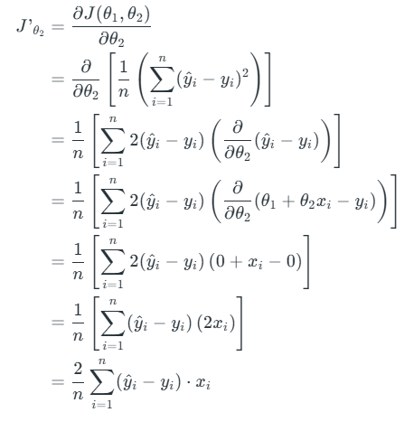
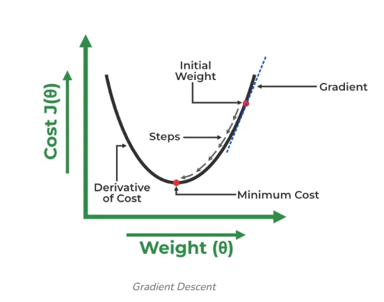
A linear regression model can be trained using the optimization algorithm gradient descent by iteratively modifying the model’s parameters to reduce the mean squared error (MSE) of the model on a training dataset. To update θ1 and θ2 values in order to reduce the Cost function (minimizing RMSE value) and achieve the best-fit line the model uses Gradient Descent. The idea is to start with random θ1 and θ2 values and then iteratively update the values, reaching minimum cost.
A gradient is nothing but a derivative that defines the effects on outputs of the function with a little bit of variation in inputs.
Let’s differentiate the cost function(J) with respect to θ1
Let’s differentiate the cost function(J) with respect to θ2
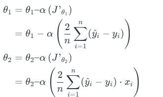
Finding the coefficients of a linear equation that best fits the training data is the objective of linear regression. By moving in the direction of the Mean Squared Error negative gradient with respect to the coefficients, the coefficients can be changed. And the respective intercept and coefficient of X will be if α is the learning rate.
Assumptions of Simple Linear Regression
Linear regression is a widely used technique for analyzing and predicting the behavior of a dependent variable. However, to ensure accuracy and reliability, certain assumptions must be met:
- Linearity:
There must be a linear relationship between the independent and dependent variables. Changes in the dependent variable should correspond proportionally to changes in the independent variable(s), forming a straight-line relationship in the data. If the relationship is not linear, linear regression will not provide an accurate model. - Independence:
The observations in the dataset should be independent of each other. This means that the value of the dependent variable for one observation does not depend on the value of another observation. Violations of this assumption reduce the accuracy of the regression model. - Homoscedasticity:
The variance of the residuals (errors) should remain constant across all levels of the independent variable(s). If the variance changes (heteroscedasticity), the model may not provide valid results. - Normality:
The residuals should follow a normal distribution. Residuals that deviate significantly from normality can compromise the reliability of the model.
Assumptions of Multiple Linear Regression
In addition to the four assumptions of simple linear regression, multiple linear regression introduces additional considerations:
- No Multicollinearity:
Independent variables should not be highly correlated with each other. High correlation makes it challenging to determine the individual effect of each variable on the dependent variable. Multicollinearity can be detected using:- Correlation Matrix: A high correlation between independent variables indicates potential multicollinearity.
- Variance Inflation Factor (VIF): A VIF value above 10 suggests strong multicollinearity.
- Additivity:
The effect of a predictor variable on the dependent variable is assumed to be independent of the values of other variables. This means there are no interactions between predictors. - Feature Selection:
Only relevant and non-redundant independent variables should be included in the model. Adding unnecessary variables can lead to overfitting and make the model harder to interpret. - Overfitting:
Overfitting occurs when the model captures noise or random fluctuations in the training data rather than the true underlying relationship. This can reduce the model's ability to generalize to new data.
Multicollinearity
Multicollinearity arises when two or more independent variables in a regression model are highly correlated. This can obscure the ability to measure the individual impact of each variable on the dependent variable.
Methods to Detect Multicollinearity:
- Correlation Matrix:
A correlation matrix highlights relationships between independent variables. High correlations (close to ±1) suggest multicollinearity. - Variance Inflation Factor (VIF):
VIF quantifies how much the variance of a regression coefficient is inflated due to multicollinearity. A VIF value above 10 is a common indicator of multicollinearity.
Linear Regression Line
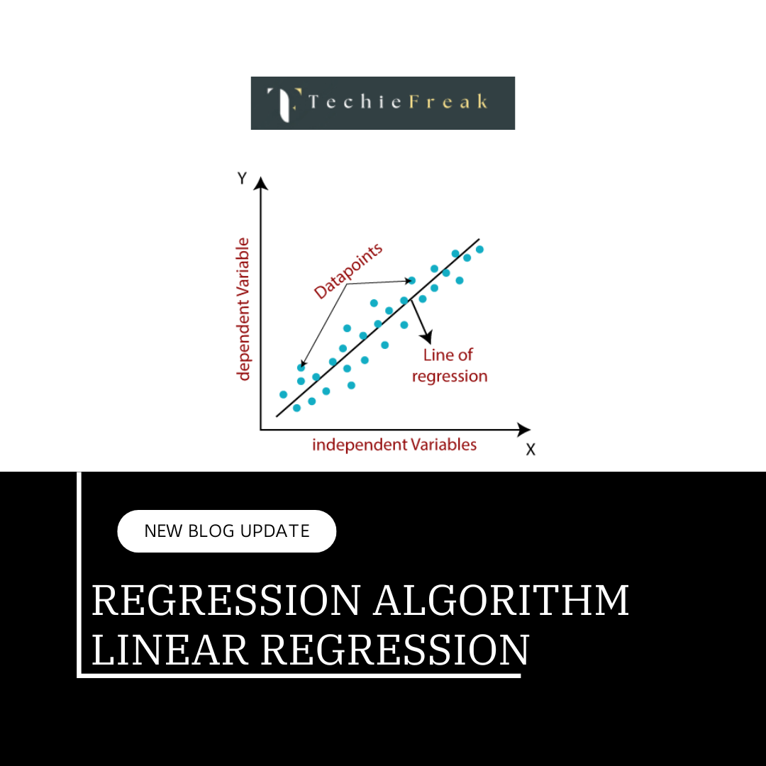
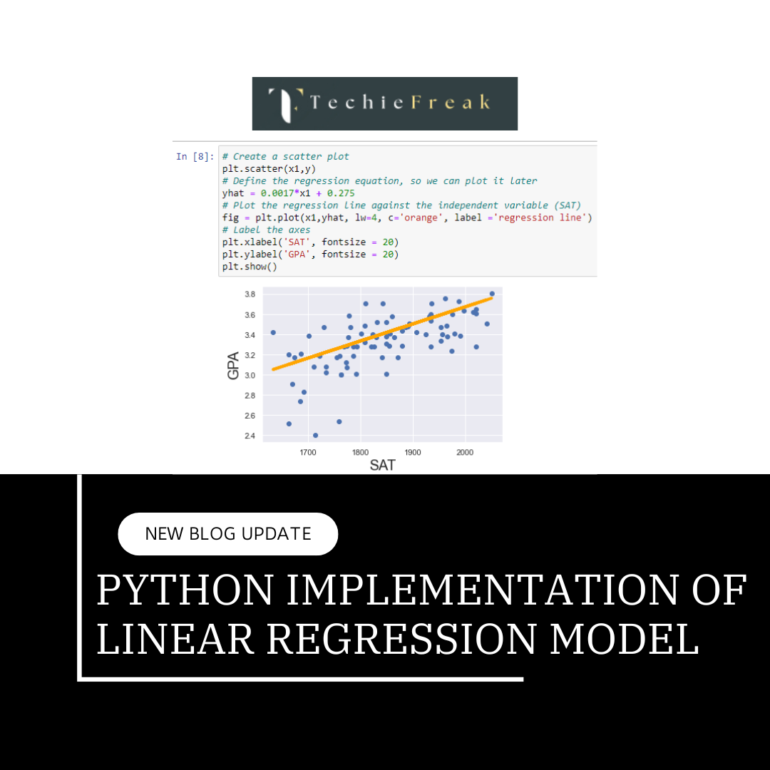
The linear regression line provides valuable insights into the relationship between the two variables. It represents the best-fitting line that captures the overall trend of how a dependent variable (Y) changes in response to variations in an independent variable (X).
- Positive Linear Regression Line: A positive linear regression line indicates a direct relationship between the independent variable (X) and the dependent variable (Y). This means that as the value of X increases, the value of Y also increases. The slope of a positive linear regression line is positive, meaning that the line slants upward from left to right.
- Negative Linear Regression Line: A negative linear regression line indicates an inverse relationship between the independent variable (X) and the dependent variable (Y). This means that as the value of X increases, the value of Y decreases. The slope of a negative linear regression line is negative, meaning that the line slants downward from left to right.
Next Topic- Python Implementation of Linear Regression Model
.png)
.png)
.png)
.png)
.png)
.png)
 Algorithm for Machine Learning.jpg)
 Algorithm.jpg)
.png)
.png)
.png)
.png)
.png)
.png)
