 Algorithm.jpg)
What is Support Vector Machine (SVM) Algorithm?
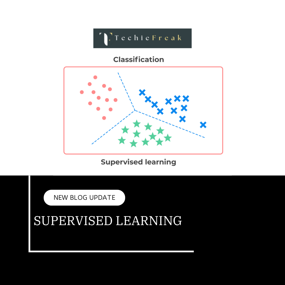
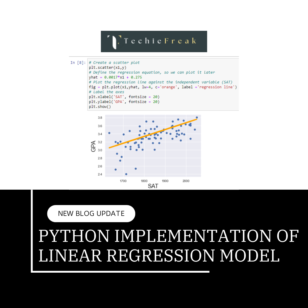
Support Vector Machine (SVM) is a supervised machine learning algorithm used for classification and regression tasks. It works by finding the optimal hyperplane that best separates data points into distinct classes in an n-dimensional space. SVM aims to maximize the margin between the hyperplane and the nearest data points from each class, called support vectors. For non-linear data, SVM uses the kernel trick to transform the data into a higher-dimensional space, making it linearly separable. With its ability to handle high-dimensional datasets and provide robust performance, SVM is widely used in applications like image classification, text categorization, and bioinformatics.
Key Idea:
SVM finds the hyperplane (decision boundary) that best separates data points of different classes in an n-dimensional space. The key is to maximize the margin (distance) between the hyperplane and the closest data points from each class, called support vectors.
Algorithm for Support Vector Machines
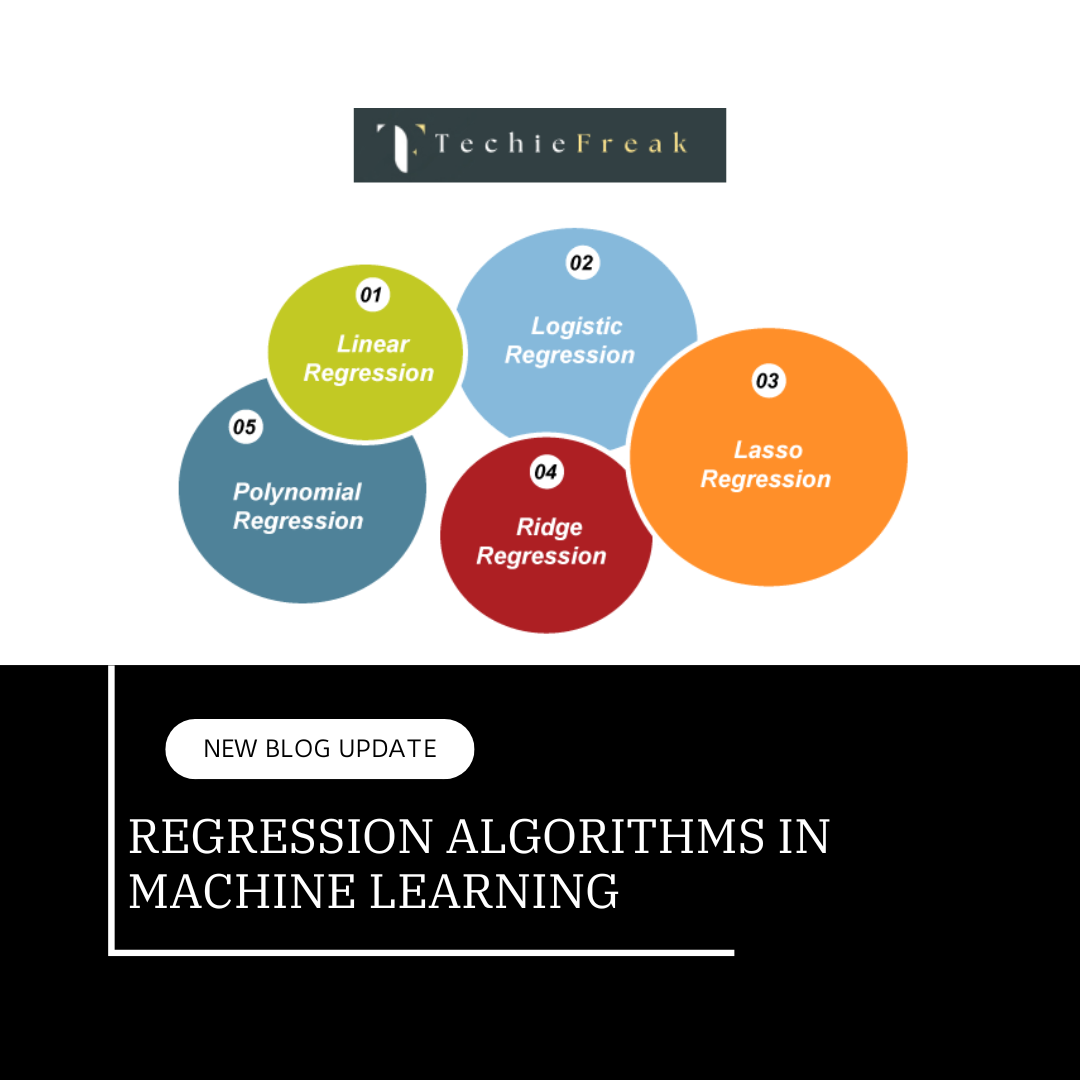
One of the most widely used supervised learning algorithms for both classification and regression problems is the Support Vector Machine, or SVM. But its main application is in machine learning for classification problems.
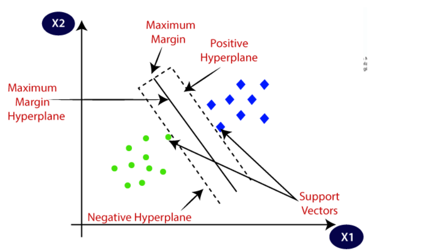
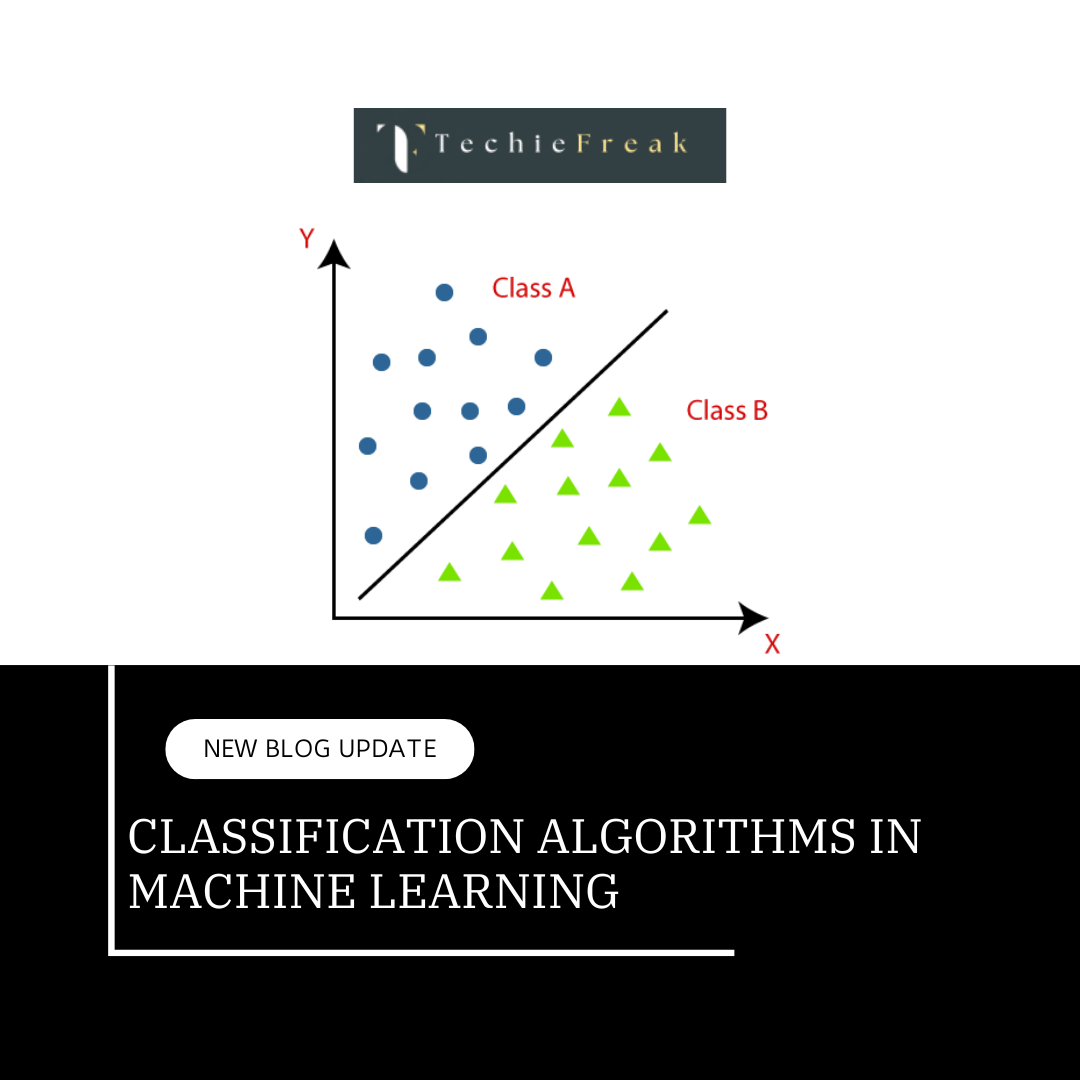
In order to make it simple to classify new data points in the future, the SVM algorithm aims to draw the optimal line or decision boundary that can divide n-dimensional space into classes. We refer to this optimal decision boundary as a hyperplane.
In order to create the hyperplane, SVM selects the extreme points and vectors. The algorithm is referred to as a Support Vector Machine because these extreme situations are known as support vectors. Examine the diagram below, which shows two distinct categories.
Why Use SVM?
- Effective in High Dimensions: SVM performs well in cases where the number of dimensions exceeds the number of samples.
- Versatility: Can handle both linear and non-linear data using kernel functions.
- Robust to Overfitting: Especially useful in scenarios with clear margin separation.
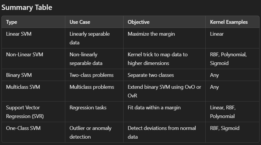
SVM types
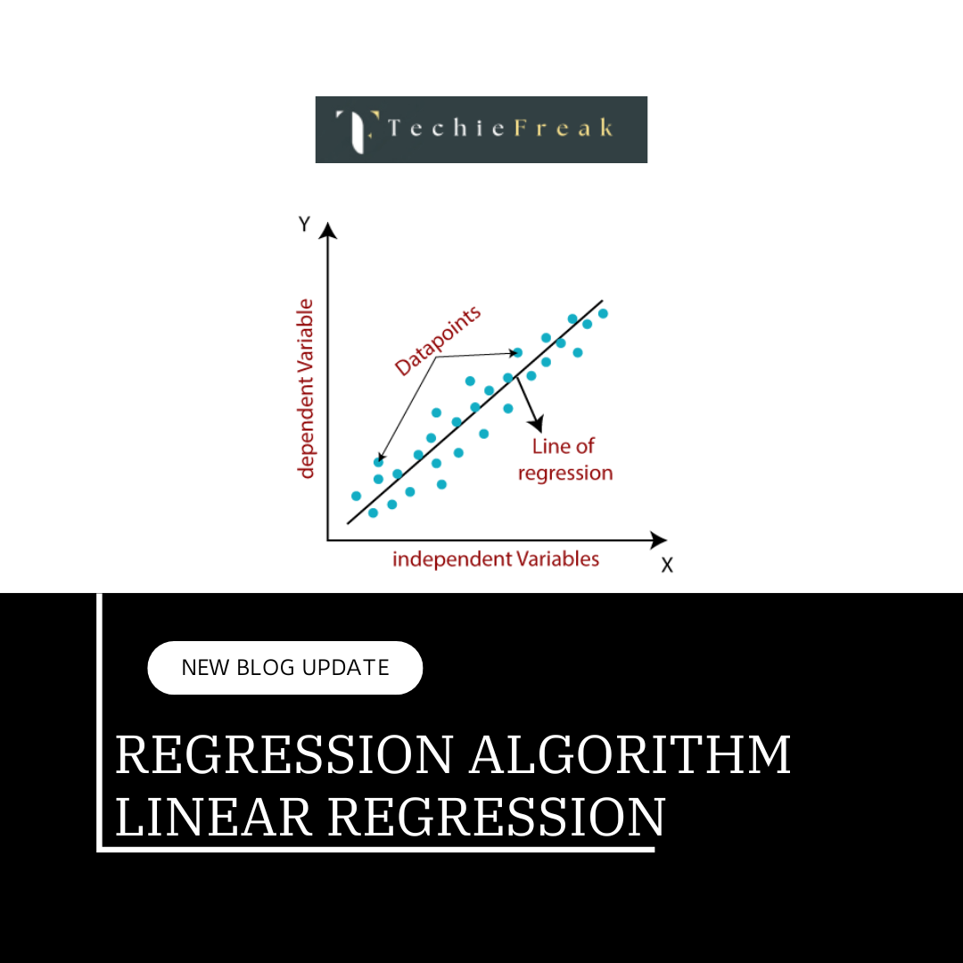
1. Linear SVM
- Use case: When the data is linearly separable, i.e., it can be separated into classes using a straight hyperplane.
- Objective: Find the best hyperplane that separates the data points of different classes with the maximum margin.
- Kernel used: Linear kernel.
Example
If we have two features like age and salary, and the data is distributed such that classes can be separated by a straight line, Linear SVM is suitable.
2. Non-Linear SVM
- Use case: When the data is not linearly separable, i.e., it cannot be separated using a straight hyperplane.
- Objective: Transform the data into a higher-dimensional space using a kernel trick so that it becomes linearly separable.
- Common kernels:
- Polynomial kernel: Maps the data into higher-degree polynomials.
- Radial Basis Function (RBF) kernel: Creates decision boundaries in infinite-dimensional spaces.
Example
If the data forms concentric circles, the RBF kernel can map it into a higher-dimensional space where it becomes linearly separable.
3. Binary SVM
- Use case: When the problem involves only two classes.
- Objective: Classify the data into one of the two classes by finding the best hyperplane that separates them.
Example
Predicting whether an email is "spam" or "not spam."
4. Multiclass SVM
- Use case: When the problem involves more than two classes.
- Objective: Extend SVM for multiclass classification problems using the following approaches:
- One-vs-One (OvO): Breaks the problem into multiple binary classification problems, one for each pair of classes. For nnn classes, n(n−1)2\frac{n(n-1)}{2}2n(n−1) classifiers are built.
- One-vs-Rest (OvR): Creates one classifier per class, treating it as a binary problem by considering one class as "positive" and the rest as "negative."
Example
Classifying images of animals into "cat," "dog," and "rabbit."
5. SVM for Regression (SVR)
- Use case: When the goal is to predict continuous output rather than discrete classes.
- Objective: Find a hyperplane that fits the data within a certain margin of tolerance. Instead of maximizing the margin, SVR minimizes prediction errors within a margin.
Example
Predicting house prices based on features like size, location, and number of rooms.
6. SVM for Outlier Detection (One-Class SVM)
- Use case: When the problem involves detecting anomalies or outliers in the data.
- Objective: Learn a decision boundary around the majority of data points and classify new data points as belonging to the class or being an outlier.
- Kernel used: Often uses RBF for mapping into higher dimensions.
Example
Detecting fraudulent transactions in banking or unusual network activity in cybersecurity.
How does Support Vector Machine Algorithm Work?
Finding the optimal decision boundary, also known as a hyperplane, that divides data points into distinct classes with the greatest margin is how the Support Vector Machine (SVM) algorithm operates. Here is a thorough breakdown of SVM's operation step-by-step:
1. Problem Setup
- SVM is used for both classification and regression, but it is most commonly applied to classification problems.
- The input data consists of:
- Features (X): The input variables (e.g., height, weight, age).
- Labels (y): The target variable (e.g., "0" or "1").
2. Hyperplane and Decision Boundary
Key Differences Between Hyperplane and Decision Boundary:
| Aspect | Hyperplane | Decision Boundary |
|---|---|---|
| Definition | A flat, n−1n-1n−1-dimensional subspace in nnn-dimensions. | A line/surface separating different classes. |
| Purpose | Used in algorithms like SVM to separate classes. | Represents the boundary for classification. |
| Complexity | Always linear. | Can be linear or non-linear. |
| Usage | Mathematical/geometrical construct. | Practical representation of classification. |
3. Maximizing the Margin
- Margin: The distance between the hyperplane and the closest data points of each class. These closest data points are called support vectors.
- SVM finds the hyperplane that maximizes this margin, ensuring better generalization and reducing the risk of misclassification.
4. Key Concepts
- Support Vectors:
- The data points closest to the hyperplane.
- These points determine the position and orientation of the hyperplane.
- Soft Margin vs. Hard Margin:
- Hard Margin: Assumes data is perfectly separable. All data points must lie on the correct side of the hyperplane.
- Soft Margin: Allows some misclassification to handle noisy and overlapping data. Controlled by a parameter CCC, which balances margin size and misclassification penalty.
- Linear Separability:
- If the data is linearly separable, SVM directly finds a straight hyperplane.
- For non-linearly separable data, SVM applies the kernel trick (explained below).
5. Kernel Trick for Non-Linear Data
- If the data cannot be separated linearly, SVM uses kernels to transform the data into a higher-dimensional space where it becomes linearly separable.
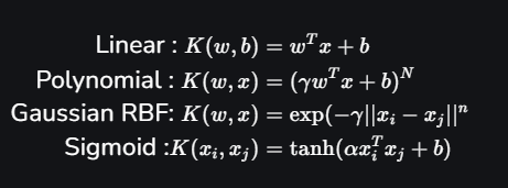
- Common kernels:
- Linear Kernel: For linearly separable data.
- Polynomial Kernel: Maps data into polynomial features.
- Radial Basis Function (RBF) Kernel: Maps data to infinite-dimensional space.
Sigmoid Kernel: Similar to a neural network activation function.
6. Mathematical Formulation
- Optimization Problem:
SVM solves the following optimization problem:
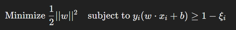
- where:
- www: Weight vector (determines the hyperplane orientation).
- bbb: Bias (determines the hyperplane position).
- ξi\xi_iξi: Slack variable (for soft margin, allowing some misclassification).
- Dual Formulation:
- Instead of solving the primal optimization problem, SVM solves its dual problem using Lagrange multipliers, making it easier to incorporate kernels.
7. Steps of SVM Algorithm
- Input: Training data with features XXX and labels yyy.
- Compute: Identify the hyperplane that separates the classes by solving the optimization problem.
- Transform: (For non-linear data) Apply the kernel function to map data into a higher-dimensional space.
- Output: A model that classifies new data points based on their position relative to the hyperplane.
8. Prediction
For a new data point xxx, the prediction is made as:
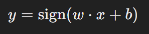
Where:
- w⋅xw \cdot xw⋅x: Measures the distance of the point from the hyperplane.
- sign\text{sign}sign: Determines the class based on whether the value is positive or negative.
9. Benefits of SVM
- works well with data that has many dimensions.
- Both linear and non-linear problems can benefit from its use.
- When there are more features than samples, it is resistant to overfitting.
10. Restrictions
- computationally costly when dealing with big datasets.
- sensitive to hyperparameters (such as kernel parameters and C) and kernel selection.
- has trouble with overlapping and noisy data.
Terminology for Support Vector Machines
- Hyperplane: In a feature space, the hyperplane is the decision boundary that divides data points of various classes. This linear equation is represented as wx+b=0 for linear classification.
- Vectors of Support: The data points that are closest to the hyperplane are called support vectors. These points are essential for figuring out the Support Vector Machine's (SVM) hyperplane and margin.
- Margin: The margin is the separation between the hyperplane and the support vector. Since a larger margin usually translates into better classification performance, the SVM algorithm's main objective is to maximize this margin.
- Kernel: In SVM, the kernel is a mathematical function that maps input data into a feature space with more dimensions. In situations where data points are not linearly separable in the original space, this enables the SVM to locate a hyperplane. The radial basis function (RBF), sigmoid, linear, and polynomial are examples of common kernel functions.
- Hard Margin: The maximum-margin hyperplane that precisely divides the data points of various classes without any misclassifications is known as a "hard margin."
- Soft Margin: SVM employs the soft margin technique when the data is not entirely separable or contains outliers. In order to balance maximizing the margin and minimizing violations, this method adds a slack variable for every data point, allowing for some misclassifications.
- C: The SVM's C parameter is a regularization term that strikes a balance between the penalty for incorrect classifications and margin maximization. A higher C value results in a smaller margin but fewer misclassifications because it enforces a harsher penalty for margin violations.
- Hinge Loss: One typical loss function in SVMs is the hinge loss. It is frequently used in conjunction with a regularization term in the objective function to penalize incorrectly classified points or margin violations.
- Dual Problem: The Lagrange multipliers connected to the support vectors are the subject of the dual problem in SVM. This formulation enables more effective computation and permits the use of the kernel trick.
Mathematical Computation: SVM
Finding the ideal hyperplane to divide data points into classes while optimizing the margin is at the heart of Support Vector Machines' (SVM) mathematical calculation. This is a thorough explanation of the SVM calculation:
1. Formulation of the Problem
The goal is to classify data points using a decision boundary defined as:
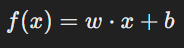
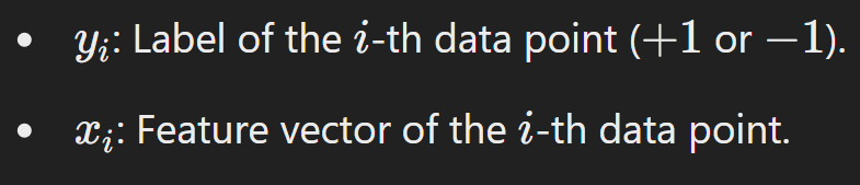
Where:
- w: Weight vector (determines the orientation of the hyperplane).
- x: Feature vector of the data point.
- b: Bias term (determines the position of the hyperplane).
For SVM:
The margin is the distance between the hyperplane and the nearest data points (support vectors). The optimal hyperplane maximizes this margin.
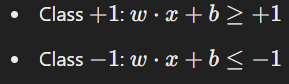
2. Objective Function
The objective function in SVM is the mathematical expression that the algorithm aims to optimize during the training process. It ensures that the SVM finds the best hyperplane that separates the data into different classes with the maximum margin while minimizing errors (if applicable).
To maximize the margin, the SVM minimizes the following:
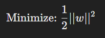
Subject to:
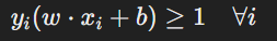
Where:
3. Soft Margin (For Non-Separable Data)
When the data is not perfectly separable, a slack variable is introduced to allow some misclassification:
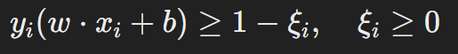
The optimization problem becomes:
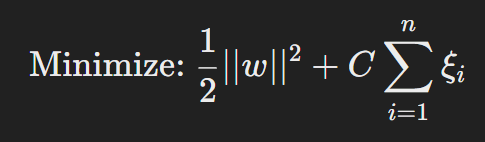
Where:
- C: Regularization parameter that balances margin maximization and misclassification.
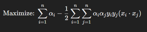
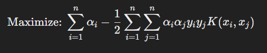
4. Dual Formulation
The primal optimization problem is converted into its dual form to make computation more efficient and incorporate kernels. The dual formulation is:
Subject to:
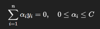
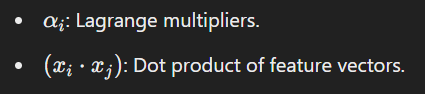
Where:
5. Kernel Trick
For non-linear problems, SVM uses a kernel function to transform data into higher-dimensional space:
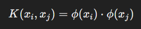
Where ϕ(x) is a mapping function. Common kernels include:
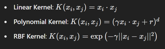
The dual formulation becomes:
6. Decision Rule
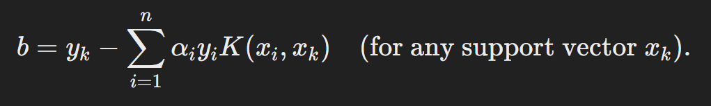
After solving for αi, the decision boundary is:
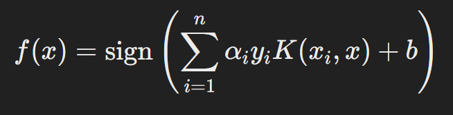
Where b is calculated using the support vectors:
Evaluating a Support Vector Machine (SVM) Model
To evaluate an SVM model, we need to assess its performance based on various metrics, depending on the type of task (classification or regression). Below are steps and metrics commonly used for evaluating an SVM model.
1. Splitting the Dataset
- Training Set: Used to train the SVM model.
- Testing Set: Used to evaluate the model's performance on unseen data.
- Validation Set (optional): For hyperparameter tuning (e.g., choosing the value of CC, kernel type, etc.).
2. Evaluation Metrics for Classification
a. Confusion Matrix
A confusion matrix shows the actual vs. predicted values in a tabular format. It contains:
- True Positives (TP): Correct positive predictions.
- True Negatives (TN): Correct negative predictions.
- False Positives (FP): Incorrect positive predictions.
- False Negatives (FN): Incorrect negative predictions.
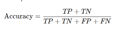
b. Accuracy
Measures the percentage of correct predictions:
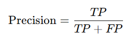
c. Precision
Measures the proportion of correctly predicted positive observations:
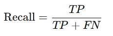
d. Recall (Sensitivity or True Positive Rate)
Measures the proportion of actual positives that are correctly identified:
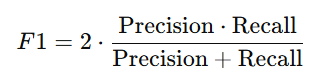
e. F1-Score
The harmonic mean of precision and recall, useful for imbalanced datasets:
f. ROC-AUC (Receiver Operating Characteristic - Area Under the Curve)
Evaluates the model's ability to distinguish between classes by plotting the True Positive Rate (TPR) against the False Positive Rate (FPR).
3. Evaluation Metrics for Regression
If the SVM is used for regression tasks (e.g., SVR), these metrics are used:
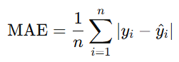
a. Mean Absolute Error (MAE)
The average absolute difference between predicted and actual values:
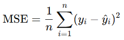
b. Mean Squared Error (MSE)
The average squared difference between predicted and actual values:
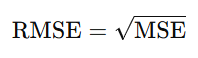
c. Root Mean Squared Error (RMSE)
The square root of MSE, providing error in the same units as the target variable:
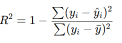
d. R-squared (R2R^2)
Measures the proportion of variance in the target variable explained by the model:
4. Cross-Validation
Why Use Cross-Validation?
Cross-validation ensures that the model generalizes well by dividing the dataset into multiple folds:
- K-Fold Cross-Validation: Splits data into KK folds and trains the model on K−1K-1 folds, testing it on the remaining fold. This process repeats KK times.
- Stratified K-Fold Cross-Validation: Ensures each fold has a similar class distribution, useful for imbalanced datasets.
Output:
The average performance metric (e.g., accuracy, F1-score, etc.) across all folds.
5. Hyperparameter Tuning
Why Tune Hyperparameters?
Hyperparameters like CC, kernel type, degree (for polynomial kernels), and γ\gamma significantly affect the SVM model's performance.
Methods for Tuning:
- Grid Search: Exhaustively searches through a specified range of hyperparameters.
- Random Search: Randomly samples hyperparameters within a range.
- Bayesian Optimization: Uses probabilistic models to find the best hyperparameters.
Evaluation During Tuning:
Use cross-validation to evaluate each hyperparameter combination.
6. Feature Scaling
SVM is sensitive to the scale of features. Apply:
- Normalization (Min-Max Scaling): Scales values between 0 and 1.
- Standardization: Scales data to have a mean of 0 and a standard deviation of 1.
7. Visualizing Model Performance
a. Decision Boundary
Visualize the decision boundary in 2D or 3D to understand how the SVM separates the classes.
b. Learning Curve
Plots training and validation performance over different dataset sizes to detect overfitting or underfitting.
Key Takeaways-
Here are the key takeaways from the blog on the Support Vector Machine (SVM) Algorithm:
- Purpose and Functionality:
- SVM is a supervised machine learning algorithm primarily used for classification, but also applicable to regression and outlier detection tasks.
- It finds the optimal hyperplane (decision boundary) that separates different classes by maximizing the margin between support vectors.
- Key Concepts:
- Hyperplane: A decision boundary that divides the feature space.
- Support Vectors: The data points that lie closest to the hyperplane and determine its position.
- Margin: The distance between the hyperplane and the closest data points from each class.
- Kernel Trick: For non-linearly separable data, kernels (like RBF, polynomial) are used to transform the data into a higher-dimensional space to make it separable.
- Types of SVM:
- Linear SVM: For linearly separable data, where a straight hyperplane can separate the classes.
- Non-linear SVM: For non-linearly separable data, using kernel functions to map data into higher dimensions.
- Binary SVM: Classifies data into two classes.
- Multiclass SVM: Extends binary SVM to handle multiple classes through approaches like One-vs-One (OvO) or One-vs-Rest (OvR).
- SVM for Regression (SVR): Used for continuous output prediction rather than discrete classes.
- SVM for Outlier Detection (One-Class SVM): Detects anomalies or outliers by classifying data points that do not belong to the main distribution.
- Working of SVM:
- Step 1: Define the problem with features (X) and labels (y).
- Step 2: Find the optimal hyperplane that maximizes the margin between classes.
- Step 3: If data is non-linearly separable, use the kernel trick to transform data into higher dimensions.
- Step 4: Make predictions based on the distance from the hyperplane.
- Benefits:
- Works well with high-dimensional data.
- Can handle both linear and non-linear problems.
- Resistant to overfitting, especially when there are more features than data points.
- Challenges and Limitations:
- Computationally expensive, especially for large datasets.
- Sensitive to hyperparameters, such as kernel and regularization (C).
- Struggles with noisy and overlapping data.
- Mathematical Formulation:
- Involves optimizing an objective function to maximize the margin and minimize classification errors.
- Uses dual formulations for efficiency, especially with kernel functions.
- Evaluation:
- For classification tasks, use metrics like accuracy, precision, recall, F1-score, and ROC-AUC.
- For regression tasks, use metrics like Mean Squared Error (MSE), Mean Absolute Error (MAE), etc.
- Common Applications:
- Image classification, text categorization, bioinformatics, anomaly detection, and regression tasks.
.png)
.png)
.png)
.png)
.png)
.png)
 Algorithm for Machine Learning.jpg)
.png)
.png)
.png)
.png)
.png)
.png)