.png)
Isomap: A Comprehensive Guide to Non-Linear Dimensionality Reduction
Isomap is a non-linear dimensionality reduction technique that combines classical multidimensional scaling (MDS) with the concept of geodesic distances. Unlike linear dimensionality reduction techniques such as Principal Component Analysis (PCA), Isomap is able to uncover the non-linear structure of data, making it suitable for data that lies on a curved manifold.
Isomap works by estimating the geodesic distances between data points and then applying classical MDS to preserve these distances in a lower-dimensional space. The result is a more faithful representation of the original data’s underlying structure, especially when the data is non-linearly distributed.
Key Concepts of Isomap
- Manifolds:
- In mathematics, a manifold is a space that locally resembles Euclidean space, but may have a more complicated global structure. For instance, the surface of a sphere is a 2D manifold in 3D space.
- Isomap operates on the assumption that high-dimensional data lies on a low-dimensional manifold, and its task is to find this manifold's lower-dimensional representation.
- Geodesic Distance:
- The geodesic distance is the shortest path between two points on a curved surface or manifold, unlike the Euclidean distance that is used in traditional methods like PCA.
- Isomap estimates geodesic distances by finding the shortest path through a neighborhood graph of data points, where each data point is connected to its nearest neighbors.
- Neighborhood Graph:
- Isomap first builds a graph where each data point is connected to its nearest neighbors. The edges in the graph represent the approximate Euclidean distances between points in the high-dimensional space.
- This graph is crucial for approximating the geodesic distances between all pairs of points in the dataset.
- Multidimensional Scaling (MDS):
- Once the geodesic distances are computed, Isomap applies classical multidimensional scaling (MDS) to the distance matrix.
- The objective of MDS is to find a low-dimensional representation of the data such that the pairwise distances between points in the lower-dimensional space are as close as possible to the geodesic distances.
How Isomap Works
The Isomap algorithm consists of the following main steps:
- Construct the Neighborhood Graph:
- Each data point is connected to its kk-nearest neighbors (or within a fixed radius).
- The graph built this way represents the data’s local structure. Each edge in the graph represents an approximation of the Euclidean distance between the points.
- Compute Geodesic Distances:
- After building the graph, the next step is to compute the geodesic distances between all pairs of points.
- These distances are estimated by finding the shortest path between points in the neighborhood graph using algorithms such as Dijkstra’s Algorithm or Floyd-Warshall Algorithm.
- Apply Classical Multidimensional Scaling (MDS):
- With the geodesic distance matrix in hand, classical MDS is applied to find a low-dimensional representation of the data.
- MDS works by trying to minimize the stress function, which measures the difference between the pairwise distances in the high-dimensional space and the low-dimensional embedding.
- Optimization:
- The optimization in MDS aims to find the positions of the data points in the lower-dimensional space that preserve the pairwise geodesic distances as much as possible.
- The result is a low-dimensional embedding of the data that reflects the manifold structure of the original data.
Mathematical Formulation of Isomap
Mathematically, Isomap can be broken down into three key steps:
- Neighborhood Graph Construction:
- Let the dataset be X={x1,x2,…,xn}}, where each xi is a point in a high-dimensional space.
- For each point xi, find its k-nearest neighbors Ni and construct a graph G, where each edge represents the Euclidean distance between xi and Ni.
- Geodesic Distance Calculation:
- Compute the geodesic distance Dij between all pairs of points xi and xj by finding the shortest path between them in the graph.
- This can be done using Dijkstra’s Algorithm or Floyd-Warshall Algorithm to find the shortest paths in the graph.
- Multidimensional Scaling (MDS):
- Given the geodesic distance matrix D, apply classical MDS to obtain the low-dimensional coordinates Y={y1,y2,…,yn}
The goal is to minimize the stress function:
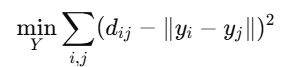
- where dij are the geodesic distances and ∥yi−yj∥ are the Euclidean distances in the low-dimensional space.
Advantages of Isomap
- Non-Linear Dimensionality Reduction:
- Isomap is capable of capturing non-linear relationships in data. Unlike linear methods like PCA, Isomap can effectively reduce the dimensionality of data that lies on non-linear manifolds.
- Geodesic Distance Preservation:
- Isomap preserves the geodesic distances between points, which is particularly useful for data that has an inherent non-Euclidean structure (e.g., data on a sphere or a torus).
- Unsupervised Learning:
- Isomap is an unsupervised technique, meaning it doesn’t require labeled data. It relies solely on the geometry of the data to uncover its intrinsic structure.
Disadvantages of Isomap
- Computational Complexity:
- Isomap can be computationally expensive, especially for large datasets. Computing pairwise distances and finding the shortest paths for all pairs of points in the dataset can be slow.
- Neighborhood Size Sensitivity:
- The performance of Isomap depends on the choice of the number of nearest neighbors kk. A small value of kk may result in an incomplete graph that doesn’t adequately represent the data's structure, while a large kk may over-smooth the data.
- Curse of Dimensionality:
- Isomap suffers from the curse of dimensionality, meaning that as the dimensionality of the data increases, the method becomes less effective. It may struggle to capture the structure of very high-dimensional datasets, especially if they are sparse.
Applications of Isomap
- Image and Object Recognition:
- Isomap is used in image recognition tasks where the data is high-dimensional (such as pixel data). By reducing the dimensionality, Isomap makes it easier to perform object recognition and classification.
- Speech and Audio Processing:
- In speech recognition, Isomap can be used to reduce the dimensionality of audio features while preserving the speech signal’s underlying structure, leading to better classification results.
- Genomics and Bioinformatics:
- In genomic data analysis, Isomap can reduce the dimensionality of gene expression data, which may have a complex non-linear structure, helping researchers uncover hidden patterns and relationships.
- Robotics and Motion Analysis:
- Isomap is applied to motion capture data, which is often high-dimensional, to analyze and model human movement or object trajectories in a lower-dimensional space.
Key Takeaways
Isomap is a powerful tool for non-linear dimensionality reduction. Its ability to preserve the geodesic distances between data points makes it suitable for tasks where the data lies on a non-linear manifold. While Isomap has its limitations, particularly with computational complexity and sensitivity to neighborhood size, it remains a valuable technique for analyzing complex datasets in fields such as computer vision, bioinformatics, and machine learning.
Understanding how Isomap works, its mathematical foundation, and its applications can help researchers and practitioners in various domains leverage this technique effectively.
.png)
.png)
.png)
.png)
.png)
.png)
.png)
.png)
.png)
.png)
.png)
.png)
.png)
.png)
.png)
.png)
.png)
.png)
.png)
.png)
.png)
.png)
.png)