.png)
Recurrent Neural Networks (RNN) and Long Short-Term Memory (LSTM) – A Detailed Theoretical Guide
Introduction
Recurrent Neural Networks (RNNs) are a class of neural networks designed for processing sequential data, such as time series, speech, text, and video. Unlike traditional feedforward networks, RNNs have an internal memory that allows them to retain information from previous inputs.
However, RNNs suffer from vanishing and exploding gradients, limiting their ability to learn long-term dependencies. To overcome this, Long Short-Term Memory (LSTM) networks were introduced, which can remember information for long periods using gated mechanisms.
1. What is a Recurrent Neural Network (RNN)?
A Recurrent Neural Network (RNN) is a type of artificial neural network specifically designed to handle sequential data by maintaining a hidden state that captures information from previous time steps. Unlike traditional feedforward neural networks, RNNs can process time-dependent patterns, making them ideal for tasks like language modeling, speech recognition, and time-series forecasting.
Why Use RNNs?
Traditional neural networks process input data independently, meaning they do not have any memory of previous inputs. This limitation makes them ineffective for sequential tasks where past information is crucial.
Examples of Sequential Tasks:
Natural Language Processing (NLP) – Predicting the next word in a sentence.
Speech Recognition – Converting spoken words into text.
Time-Series Forecasting – Stock price prediction, weather forecasting.
Machine Translation – Translating text from one language to another.
RNNs solve this problem by incorporating a looping mechanism, where each step's output is influenced by previous steps. This enables the network to retain memory of past inputs.
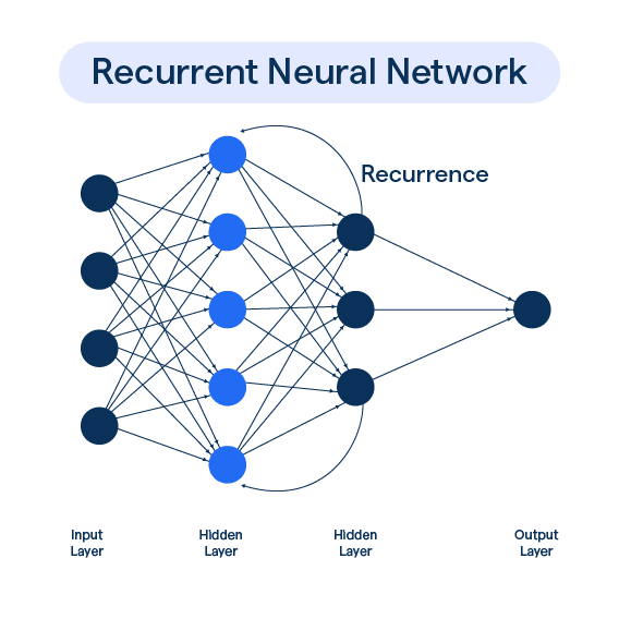
2. How RNNs Work
Mathematical Representation
At each time step t, an RNN receives:
- Input (xt) – Current time step input
- Hidden State (ht) – Captures past information
- Output (yt) – Predicted output
The hidden state is updated as:
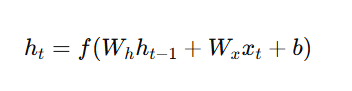
Where:
- ht = Current hidden state
- ht−1 = Previous hidden state
- Wh,Wx= Weight matrices
- b = Bias
- f = Activation function (commonly tanh or ReLU)
The final output is:
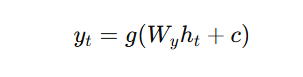
Where:
- g is often a softmax function (for classification tasks).
3. Challenges of RNNs
Despite their effectiveness, RNNs face three major challenges:
1. Vanishing Gradient Problem
- When training deep RNNs, gradients become extremely small (close to zero) and stop updating weights, preventing learning from long-term dependencies.
- This occurs when using activation functions like sigmoid and tanh, which squash values between 0 and 1 or -1 and 1, leading to gradient shrinkage.
2. Exploding Gradient Problem
- If gradients become too large, weights grow exponentially, leading to instability.
- This often happens with large sequences and high learning rates.
3. Short-Term Memory
- RNNs struggle to remember long-term dependencies in sequential data.
- This is a major limitation in applications like long text understanding or video processing.
To address these challenges, LSTM networks were introduced.
4. Long Short-Term Memory (LSTM) Networks – Introduction
LSTMs are a special type of RNN designed to overcome vanishing gradients and retain information for long periods.
How?
- LSTMs use a memory cell and gates to control what to keep and what to forget from past inputs.
- Unlike standard RNNs, LSTMs selectively retain important information and discard irrelevant data.
5. LSTM Architecture and Gates
Long Short-Term Memory (LSTM) networks are a special type of Recurrent Neural Network (RNN) designed to overcome the vanishing gradient problem and better handle long-term dependencies in sequential data.
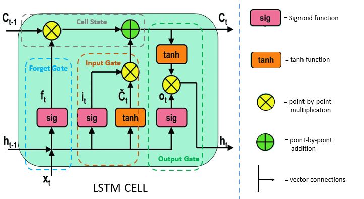
Each LSTM unit consists of:
- Cell State (Ct) – Stores long-term information.
- Hidden State (ht) – Short-term memory for the current time step.
- Gates – Control what information flows through:
- Forget Gate (ft) – Decides what to remove.
- Input Gate (it) – Decides what to add.
- Output Gate (ot) – Controls the final output.
Mathematical Equations of LSTM
Forget Gate
The forget gate determines whether past information should be retained or discarded based on the current input and previous hidden state.
- Determines whether to keep or discard previous memory.
- A sigmoid function decides which part of the previous cell state (Ct−1) should be forgotten.
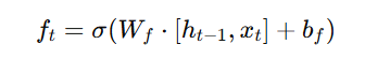
Where:
- ft is the forget gate output (values between 0 and 1).
- Wf are learned weights.
- ht−1 is the previous hidden state.
- xt is the current input.
- bf is the bias.
If ft is close to 1 → Keep past information.
If ft is close to 0 → Forget past information.
Input Gate
The input gate decides what new information should be stored in the cell state by filtering important data through a combination of sigmoid and tanh functions.
- Determines which new information to store in the cell state.
- Uses a sigmoid function to filter important input information and a tanh function to create candidate values for storage.
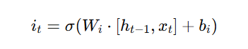
- Controls what new information is added.
Cell State Update
The cell state is the core memory of an LSTM, responsible for carrying long-term information across time steps. It is updated at each step by combining past memory with new relevant information. This update process is controlled by the forget gate and the input gate. The forget gate determines how much of the previous cell state should be retained, while the input gate decides what new information should be added.
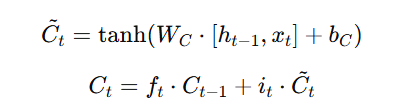
- Where:
- it decides how much new information to add.
- Ct~ is the candidate value (a new memory to store).
Combines past and new memories.
Output Gate
The output gate regulates what information is passed to the next time step by controlling how much of the updated cell state contributes to the final hidden state.
- Controls what the hidden state (ht) should be.
- Uses a sigmoid function to determine how much of the updated cell state should be passed as the output.
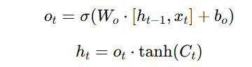
- Where:
- ot decides how much information from the cell state is passed to the hidden state.
- ht is the final hidden state, which carries short-term memory to the next time step.
- Determines the final hidden state output.
By using these gates, LSTMs can retain long-term dependencies, making them ideal for speech recognition, machine translation, and time-series forecasting.
6. Key Differences: RNN vs. LSTM
| Feature | RNN | LSTM |
|---|---|---|
| Memory Type | Short-term | Long-term |
| Vanishing Gradient Problem | Yes | No |
| Gates | None | Forget, Input, Output |
| Training Complexity | Lower | Higher |
| Performance on Long Sequences | Poor | Excellent |
LSTMs extend RNNs by adding gates to control memory flow, making them more effective for long-sequence tasks.
7. Applications of RNNs and LSTMs
1. Natural Language Processing (NLP)
- Sentiment analysis
- Text generation (e.g., chatbots)
- Machine translation (e.g., Google Translate)
2. Speech Recognition
- Virtual assistants (e.g., Siri, Alexa)
- Voice-based authentication
3. Time-Series Forecasting
- Stock price prediction
- Weather forecasting
4. Video Analysis
- Human action recognition
- Video captioning
5. Healthcare Applications
- Predicting disease progression
- Analyzing medical records
8. Challenges and Solutions in RNNs & LSTMs
| Challenge | Solution |
|---|---|
| Long training times | Use GPU acceleration |
| Exploding gradients | Use gradient clipping |
| Vanishing gradients | Use LSTM or GRU |
| High memory requirements | Optimize model architecture |
Key Takeaways:
RNNs retain memory through hidden states but struggle with long-term dependencies.
LSTMs solve this using gates to selectively store and forget information.
LSTMs outperform RNNs in handling long sequences and vanishing gradients.
Applications include NLP, speech recognition, stock prediction, and healthcare.
Next Blog- Python Implementation of Recurrent Neural Networks
.png)
.png)
.png)
.png)
.png)
.png)
.png)
.png)
.png)
.png)
.png)
.png)
.png)
.png)