.png)
Convolutional Neural Networks (CNN)
Introduction
Convolutional Neural Networks (CNNs) are a specialized type of neural network designed for processing structured grid data, particularly images and videos. CNNs have revolutionized the field of computer vision, enabling tasks like image classification, object detection, facial recognition, and medical image analysis.
CNNs are inspired by the way the human visual cortex processes images. Instead of treating an image as a single set of input values, CNNs extract features such as edges, textures, and patterns using convolution operations.
1. CNN Architecture and Components
A CNN typically consists of the following layers:
- Convolutional Layer – Extracts features from input images using filters (kernels).
- Activation Function – Introduces non-linearity to help detect complex patterns.
- Pooling Layer – Reduces dimensionality while retaining important features.
- Fully Connected Layer – Connects extracted features to the output layer.
- Output Layer – Produces predictions (e.g., class probabilities in image classification).
These layers work together to detect and classify features in an image, from simple edges to complex objects.
2. Convolutional Layers and Filters
What is Convolution?
Convolution is the fundamental operation in CNNs. It involves sliding a small filter (kernel) over the input image and computing the dot product between the filter and a region of the image.
Mathematically, convolution is represented as:
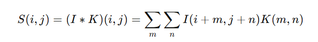
Where:
- I = Input image
- K = Kernel (filter)
- S = Output feature map
Role of Filters (Kernels) in Convolutional Neural Networks (CNNs)
Filters, also known as kernels, are small matrices that slide over an input image to extract meaningful features. They play a crucial role in feature detection, enabling Convolutional Neural Networks (CNNs) to recognize patterns such as edges, textures, and shapes. The learned filters help CNNs generalize across different images.
Types of Filters:
- Edge Detection Filters:
- Used to identify edges and boundaries in an image by detecting abrupt intensity changes.
- Examples: Sobel, Prewitt, and Canny filters.
- Sharpening Filters:
- Enhance the details in an image by amplifying high-frequency components.
- Example: Laplacian filter.
- Blurring Filters (Smoothing Filters):
- Reduce image noise and smooth out variations in intensity.
- Examples: Gaussian blur, Average filter.
- Embossing Filters:
- Create a 3D effect by highlighting edges in a specific direction.
- Gabor Filters:
- Used for texture analysis and feature extraction, often in facial recognition tasks.
How CNNs Learn Filters
Unlike traditional image processing techniques where filters are manually designed, CNNs automatically learn optimal filters during training. Through backpropagation and gradient descent, the network adjusts filter values to minimize error, ensuring the extracted features are useful for classification, detection, or segmentation tasks.
Each layer of a CNN applies multiple filters to an input image, detecting simple features like edges in the early layers and more complex patterns like textures and objects in deeper layers.
Mathematical Example of Convolution in CNNs
Let's walk through a simple example of convolution using a 3x3 filter (kernel) on a 5x5 input image. The filter slides over the image to detect features like edges, and at each step, it performs element-wise multiplication followed by summation.
Step 1: Define the Input Image (5x5 matrix)
For simplicity, let's consider a grayscale image where each pixel has a value between 0 (black) and 255 (white):
Input Image:
[[ 1, 2, 3, 0, 1],
 [ 4, 5, 6, 1, 2],
 [ 7, 8, 9, 2, 3],
 [ 0, 1, 2, 3, 4],
 [ 5, 6, 7, 8, 9]]
Step 2: Define the Filter (3x3 kernel)
Now, we'll use a Sobel filter for edge detection, which is commonly used to detect horizontal edges. The Sobel filter is:
Sobel Filter (Kernel):
[[ -1, 0, 1],
 [ -2, 0, 2],
 [ -1, 0, 1]]
Step 3: Perform Convolution
The filter moves (slides) across the input image, performing the following steps:
- Place the filter on the top-left 3x3 portion of the image.
- Multiply each element of the filter by the corresponding element of the image.
- Sum the results of the element-wise multiplication.
- Store the result in the output feature map.
Let’s compute the first value in the output matrix by applying the filter to the top-left corner of the input image.
First convolution (top-left 3x3 window of the image):
Image Submatrix (top-left 3x3):
[[1, 2, 3],
 [4, 5, 6],
 [7, 8, 9]]

Sobel Filter:
[[ -1,  0,  1],
 [ -2,  0,  2],
 [ -1,  0,  1]]
Now, we multiply each corresponding element and sum:
(1 * -1) + (2 * 0) + (3 * 1) +
(4 * -2) + (5 * 0) + (6 * 2) +
(7 * -1) + (8 * 0) + (9 * 1)

= -1 + 0 + 3 - 8 + 0 + 12 - 7 + 0 + 9
= 8
So, the value at the top-left of the output feature map is 8.
Step 4: Slide the Filter Across the Image
Next, we slide the filter one step to the right and repeat the multiplication and summation for each position. This process continues until the entire image has been processed.
For the next step (convolution at position (1, 1)):
We slide the filter to cover the next 3x3 region of the image and perform the same process:
Image Submatrix (next 3x3):
[[2, 3, 0],
 [5, 6, 1],
 [8, 9, 2]]

Sobel Filter:
[[ -1,  0,  1],
 [ -2,  0,  2],
 [ -1,  0,  1]]
The sum is:
(2 * -1) + (3 * 0) + (0 * 1) +
(5 * -2) + (6 * 0) + (1 * 2) +
(8 * -1) + (9 * 0) + (2 * 1)

= -2 + 0 + 0 - 10 + 0 + 2 - 8 + 0 + 2
= -16
Thus, the value at position (1, 1) of the output feature map is -16.
Step 5: Output Feature Map
After applying the filter across all positions, the resulting output feature map (after one pass of convolution) would look like this (with more values calculated similarly):
Output Feature Map:
[[ 8, -16, ...],
 [ 4, -14, ...],
 [...]]
Final Note: Stride and Padding
- Stride determines how much the filter moves at each step. In this example, the stride is 1 (moving one pixel at a time).
- Padding is when the input image is padded with zeros around the border to ensure the output feature map has the same spatial dimensions as the input (or controlled dimensions).
Stride and Padding in Convolutional Neural Networks (CNNs)
Stride and padding are two crucial parameters that impact how a filter (kernel) moves across an image and determines the size of the output feature map.
1. Stride (Step Size of the Filter)
Stride controls how far the filter moves after each step.
- Stride = 1 → The filter moves one pixel at a time (default case).
- Stride = 2 → The filter moves two pixels at a time, reducing the output size.
Example of Stride
Consider a 5×5 input image and a 3×3 filter:
With Stride = 1
- The filter moves one pixel at a time.
- The output feature map size is (5 - 3) / 1 + 1 = 3 × 3.
With Stride = 2
- The filter moves two pixels at a time.
- The output feature map size is (5 - 3) / 2 + 1 = 2 × 2.
- This reduces computation but may lose finer details.
Effect of Larger Strides
- Reduces the spatial dimensions of the feature map.
- Reduces computational cost.
- May cause loss of important details if stride is too large.
2. Padding (Adding Extra Pixels Around the Image)
When a filter moves over an image, it shrinks the spatial dimensions. To prevent this, we use padding, which adds extra pixels (usually zeros) around the image borders.
Types of Padding
- Valid Padding ("No Padding")
- No extra pixels are added.
- The feature map size decreases.
- Formula: Output Size=(N−F)S+1\text{Output Size} = \frac{(N - F)}{S} + 1 where N = input size, F = filter size, S = stride.
- Same Padding ("Zero Padding")
- Zeros are added to the borders so the output size remains the same as the input.
- Ensures that every pixel in the input gets a chance to contribute.
- Formula: P=(F−1)2P = \frac{(F - 1)}{2} where P = padding size.
Example of Padding
Consider a 5×5 input image with a 3×3 filter.
Without Padding (Valid Padding)
Input (5x5):
[ 1  2  3  4  5 ]
[ 6  7  8  9 10 ]
[11 12 13 14 15 ]
[16 17 18 19 20 ]
[21 22 23 24 25 ]
- After applying a 3×3 filter, the output size is 3×3.
With Same Padding (Padding = 1)
Padded Input (7x7):
[ 0  0  0  0  0  0  0 ]
[ 0  1  2  3  4  5  0 ]
[ 0  6  7  8  9 10  0 ]
[ 0 11 12 13 14 15  0 ]
[ 0 16 17 18 19 20  0 ]
[ 0 21 22 23 24 25  0 ]
[ 0  0  0  0  0  0  0 ]
- Now, applying a 3×3 filter will maintain the 5×5 output size.
Effect of Padding
- Preserves spatial dimensions of the input.
- Helps extract features near image edges.
- Prevents excessive shrinking of feature maps in deep networks.
3. Pooling Layers
What is Pooling?
Pooling is a downsampling technique that reduces the size of feature maps by summarizing regions of pixels into a single value. Instead of analyzing every pixel individually, pooling focuses on the most important features, improving efficiency and robustness.
Key Benefits of Pooling:
- Reduces Computational Cost: Fewer computations by reducing feature map size.
- Enhances Translation Invariance: Small shifts in the input image won’t drastically affect results.
- Prevents Overfitting: Reduces the amount of information, making the network more generalizable.
Types of Pooling
There are three major types of pooling used in CNNs:
(a) Max Pooling
Max pooling selects the maximum value from each region of the feature map.
Example
Consider a 4×4 feature map and a 2×2 max pooling operation:
Before Max Pooling (4×4 feature map):
1   3   2   4
5   6   8   9
2   4   1   3
7   5   6   8
After applying 2×2 Max Pooling:
6   9
4   8
Advantages of Max Pooling:
- Captures the most prominent feature in each region.
- Helps retain important edge and texture details.
- Reduces noise by focusing on strong activations.
(b) Average Pooling
Average pooling computes the mean value of each region.
Example
Using a 2×2 average pooling on the same feature map:
Before Average Pooling:
1   3   2   4
5   6   8   9
2   4   1   3
7   5   6   8
After 2×2 Average Pooling:
3.75   5.75
4.5    4.5
Advantages of Average Pooling:
- Retains overall information by considering all pixels.
- Useful for tasks where general patterns are more important than sharp edges.
- Less aggressive than max pooling, preserving more details.
(c) Global Pooling
Global pooling reduces the entire feature map into a single value per channel, typically by applying max pooling or average pooling over the entire feature map.
Example of Global Average Pooling:
If we have a 7×7 feature map, Global Average Pooling takes the mean of all 49 values and returns a single value.
Uses of Global Pooling:
- Often used in the final layers of a CNN before classification.
- Reduces dimensionality to 1 value per feature map, making it more compact.
- Works well in architectures like GoogLeNet and ResNet for classification tasks.
Pooling Parameters: Stride and Pool Size
Pooling layers have two important parameters:
- Pool Size (k×k) – Determines the size of the region (e.g., 2×2 or 3×3).
- Stride (s) – Determines the step size for moving the pooling window.
For example, a 2×2 max pooling with stride = 2 reduces a 4×4 feature map to 2×2.
| Pool Size | Stride | Output Size (from 4×4) |
|---|---|---|
| 2×2 | 2 | 2×2 |
| 2×2 | 1 | 3×3 |
| 3×3 | 1 | 2×2 |
Choosing the Right Pooling Method
| Pooling Type | Best For |
|---|---|
| Max Pooling | Detecting edges, textures, and prominent features. |
| Average Pooling | Retaining global information and reducing noise. |
| Global Pooling | Compact feature representation for classification. |
4. Fully Connected Layers
After convolution and pooling, extracted features are fed into fully connected layers (FC layers).
- Each neuron in an FC layer receives input from all neurons in the previous layer.
- FC layers transform extracted features into class scores using weights and biases.
- The final FC layer typically uses the softmax function to produce class probabilities.
5. Activation Functions in CNNs
Activation functions introduce non-linearity, allowing CNNs to learn complex patterns. Common activation functions used in CNNs include:
- ReLU (Rectified Linear Unit)
- Formula: f(x)=max(0,x)
- ReLU is the most widely used activation function in CNNs because it prevents the vanishing gradient problem.
- Leaky ReLU
- Allows a small negative slope instead of setting negative values to zero.
- Helps in cases where ReLU neurons "die" (output remains zero).
- Softmax
- Used in the output layer for multi-class classification.
- Converts scores into probabilities.
6. CNN Training Process
1. Forward Propagation
- The input image passes through convolutional layers, activation functions, pooling layers, and fully connected layers to generate an output prediction.
2. Loss Calculation
- The output is compared with the actual label using a loss function such as cross-entropy loss (for classification).
3. Backpropagation and Weight Updates
- The error is propagated backward using the chain rule of calculus.
- Weights in convolutional and fully connected layers are updated using gradient descent (e.g., Adam, RMSprop).
4. Iteration and Convergence
- The process repeats over multiple epochs until the network learns to minimize the loss.
7. Common CNN Architectures
Several CNN architectures have been developed to achieve state-of-the-art performance in image tasks.
1. LeNet-5 (1998)
- One of the earliest CNNs, designed for digit recognition.
2. AlexNet (2012)
- Introduced ReLU activation and dropout to prevent overfitting.
3. VGGNet (2014)
- Used small 3×3 filters stacked together for better feature extraction.
4. GoogLeNet (Inception)
- Introduced Inception modules for efficient computation.
5. ResNet (2015)
- Introduced residual connections to address the vanishing gradient problem in deep networks.
8. Applications of CNNs
1. Image Classification
- Identifying objects in images (e.g., cat vs. dog).
2. Object Detection
- Used in autonomous vehicles and security systems.
3. Face Recognition
- Used in biometrics (e.g., Apple Face ID).
4. Medical Image Analysis
- Detecting tumors, cancers, and other medical conditions from X-rays and MRIs.
5. Self-Driving Cars
- CNNs analyze real-time images to detect pedestrians, traffic signals, and obstacles.
9. Challenges and Solutions in CNNs
1. Computational Cost
- Solution: Use hardware accelerators like GPUs and TPUs.
2. Overfitting
- Solution: Data augmentation, dropout, and regularization techniques.
3. Limited Training Data
- Solution: Use transfer learning with pre-trained models.
Key Takeaways:
- CNNs consist of convolutional layers, pooling layers, and fully connected layers.
- Filters (kernels) extract patterns from images.
- Activation functions (ReLU, Softmax) introduce non-linearity.
- Backpropagation and gradient descent train CNNs efficiently.
- CNNs power applications like image recognition, object detection, and self-driving cars.
Next Blog- Python Implementation of Convolutional Neural Networks (CNN)
.png)
.png)
.png)
.png)
.png)
.png)
.png)
.png)
.png)
.png)
.png)
.png)
.png)
.png)