.png)
Backpropagation and Gradient Descent
Introduction
Neural networks are powerful models capable of learning from data, but they require an effective way to adjust their parameters to minimize error. Backpropagation and Gradient Descent are the two fundamental techniques that make this possible.
- Backpropagation: The method used to compute the error gradient and distribute it through the network.
- Gradient Descent: The optimization algorithm that updates the weights to minimize the error.
Understanding these concepts is crucial for anyone looking to master deep learning. Let's explore them in depth.
1. Understanding Backpropagation
What is Backpropagation?
Backpropagation, short for backward propagation of errors, is a method used to compute gradients for updating weights in a neural network. It is based on the chain rule of calculus, allowing information to flow backward from the output layer to the input layer, adjusting weights at each step.
It answers two key questions:
- How much does each weight contribute to the final error?
- How should each weight be updated to reduce the error?
Why is Backpropagation Needed?
A neural network consists of multiple layers, each transforming input data through a series of operations. To train such networks effectively, we need a way to efficiently distribute errors across all layers.
Backpropagation solves this problem by:
- Computing the loss function to measure the network’s performance.
- Propagating errors backward through the layers using derivatives.
- Updating the weights using optimization methods like gradient descent.
Without backpropagation, training deep networks would be infeasible due to inefficient weight adjustments.
Mathematical Foundation of Backpropagation
To understand backpropagation, let’s break it down step by step:
- Forward Pass: The input is passed through the network, and the output is computed using activation functions like sigmoid, ReLU, or softmax.
- Compute the Loss: The difference between the predicted and actual values is calculated using a loss function like Mean Squared Error (MSE) or Cross-Entropy Loss.
- Backward Pass: The error is propagated backward using the chain rule, calculating the gradient of the loss with respect to each weight.
- Update the Weights: The computed gradients are used to adjust the weights in the network to reduce the error.
2. Understanding Gradient Descent
What is Gradient Descent?
Gradient Descent is an optimization algorithm used to minimize the loss function by adjusting the weights in the direction that reduces error. It is based on the idea that the gradient (or derivative) of a function points in the direction of the steepest ascent.
Since we want to minimize the loss, we take steps in the opposite direction of the gradient.
Mathematically, the weight update is given by:
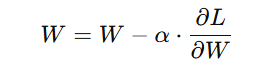
Where:
- W = weight to be updated
- α = learning rate (controls the step size)
- ∂L/∂W= gradient of the loss function
This process is repeated iteratively until the loss function reaches a minimum.
3. Types of Gradient Descent
There are three main types of gradient descent, each with its own advantages and trade-offs:
1. Batch Gradient Descent
- Computes the gradient using the entire dataset at each iteration.
- Advantage: Converges smoothly since it considers all data.
- Disadvantage: Computationally expensive for large datasets.
2. Stochastic Gradient Descent (SGD)
- Computes the gradient using only one random data point at a time.
- Advantage: Faster updates and better generalization.
- Disadvantage: Noisy updates lead to instability.
3. Mini-Batch Gradient Descent
- Uses a subset of data (mini-batch) to compute gradients.
- Advantage: Balances stability (batch) and efficiency (SGD).
- Disadvantage: Requires selecting an appropriate mini-batch size.
4. The Role of the Learning Rate
The learning rate (α) is a crucial hyperparameter in gradient descent.
- If α is too small: The network learns very slowly and might get stuck in local minima.
- If α is too large: The network may overshoot the minimum, leading to divergence.
Solution? Adaptive Learning Rate Methods
To avoid manual tuning of the learning rate, we use advanced optimization techniques like:
- Momentum-Based Gradient Descent
- Uses past gradients to smooth weight updates, reducing oscillations.
- RMSprop (Root Mean Square Propagation)
- Adapts the learning rate dynamically for each parameter.
- Adam (Adaptive Moment Estimation)
- Combines momentum and RMSprop, making learning more efficient.
Challenges in Backpropagation and Gradient Descent
1. Vanishing Gradient Problem
"Vanishing" means getting smaller and smaller until it's almost zero. "Gradient" refers to the small changes used to adjust weights in a neural network.
Explanation:
- In deep networks, when backpropagation calculates gradients, they shrink as they go backward through the layers.
- This means earlier layers (closer to input) receive almost no updates, making it hard for the model to learn properly.
Example:
Imagine you are passing a message through multiple people, but each person speaks more softly. By the time it reaches the first person, it’s barely audible (like the gradient disappearing).
Solution:
✔ Use ReLU activation function, which avoids this issue since its gradient is either 1 or 0, not small fractions.
✔ Use batch normalization to keep values in a stable range.
2. Exploding Gradient Problem
"Exploding" means growing too large uncontrollably. This happens to gradients when training deep networks.
Explanation:
- In deep networks, gradients multiply as they move backward. If they keep increasing, they can become so large that the model's training becomes unstable.
- The loss value may jump to NaN (not a number) or diverge instead of improving.
Example:
Imagine a microphone with too much volume—it creates a loud, distorted noise instead of clear sound. Similarly, when gradients explode, the model loses control and stops learning properly.
Solution:
✔ Gradient Clipping – Set a maximum limit for gradients.
✔ Batch Normalization – Keeps values stable.
✔ Weight Regularization (L2 penalty) – Prevents weights from becoming too large.
3. Getting Stuck in Local Minima
"Local minimum" is a small dip in the loss function where the model gets stuck, instead of finding the global minimum (best solution).
Explanation:
- The loss function of a neural network is like a bumpy surface with many valleys.
- The optimizer may find a small valley (local minimum) and stop there, thinking it's the best solution, but a deeper valley (global minimum) may exist nearby.
Example:
Imagine hiking in a foggy mountain range. You reach a small dip and think it's the lowest point, but a bigger valley is just ahead—if only you could see it!
Solution:
✔ Use Momentum Optimizers (Adam, RMSprop) to push past small valleys.
✔ Increase training data so the model generalizes better.
✔ Use learning rate scheduling, so the model can explore more.
4. Slow Convergence
"Convergence" means reaching the best solution. If it’s slow, the model takes too long to learn.
Explanation:
- If the learning rate is too small, updates are tiny, making training very slow.
- Poor weight initialization can also lead to inefficient updates.
Example:
Imagine filling a jar with water using a teaspoon—it will take forever! Similarly, a small learning rate makes tiny changes that slow down training.
Solution:
✔ Use adaptive optimizers like Adam or RMSprop, which adjust learning rates dynamically.
✔ Use learning rate scheduling to start fast and slow down later.
✔ Use better weight initialization (Xavier/He Initialization) to start training at a better position.
5. Saddle Points
A "saddle point" is a flat region in the loss function where the gradient becomes very small, making progress slow.
Explanation:
- Unlike local minima, a saddle point has gradients that go in different directions (some increase, some decrease).
- The optimizer gets stuck because it doesn’t know which way to go.
Example:
Imagine balancing a ball on the middle of a saddle—it can roll in different directions, but at the center, it stays almost still. The optimizer struggles in this situation.
Solution:
✔ Use momentum-based optimizers (NAG, Adam) to push past saddle points.
✔ Introduce randomness (Dropout, Learning Rate Decay) to avoid getting stuck.
| Problem | What Happens? | Solution |
|---|---|---|
| Vanishing Gradient | Gradients become too small → slow learning | Use ReLU, batch normalization |
| Exploding Gradient | Gradients become too large → unstable learning | Use gradient clipping, batch norm, L2 regularization |
| Local Minima | Model gets stuck in a small valley | Use Adam optimizer, more data, learning rate scheduling |
| Slow Convergence | Training takes too long | Use adaptive optimizers, better weight initialization |
| Saddle Points | Flat regions slow down learning | Use momentum-based optimizers, add randomness |
6. Advanced Optimization Techniques
To overcome the challenges of standard gradient descent, researchers have developed several improvements:
1. Adaptive Gradient Algorithms
- Adagrad: Adapts the learning rate based on past updates, helpful for sparse data.
- Adadelta: Addresses Adagrad’s limitations by restricting learning rate changes.
- Adam: Combines momentum and adaptive learning rate techniques for faster convergence.
2. Second-Order Methods
- Newton’s Method: Uses second-order derivatives to find the optimal weight updates.
- L-BFGS (Limited-memory Broyden–Fletcher–Goldfarb–Shanno): An advanced optimization method used in small-scale deep learning problems.
Key Takeaways
- Backpropagation is essential for training deep neural networks
- It efficiently computes the gradient of the loss function.
- Gradient Descent is the core optimization algorithm in deep learning
- It updates weights by moving in the direction that reduces the loss.
- Different types of gradient descent have trade-offs
- Batch: More stable but slower.
- Stochastic: Faster but noisier.
- Mini-Batch: A balance between both.
- Challenges like vanishing gradients and local minima exist
- Using better activation functions (ReLU), optimization techniques (Adam), and regularization methods can help.
- Advanced optimizers improve learning efficiency
- Techniques like Adam, RMSprop, and Momentum help speed up convergence.
.png)
.png)
.png)
.png)
.png)
.png)
.png)
.png)
.png)
.png)
.png)
.png)
.png)
.png)