.png)
Multi-Layer Perceptron (MLP) – A Comprehensive Guide
Introduction to MLP
A Multi-Layer Perceptron (MLP) is an artificial neural network (ANN) that consists of multiple layers of neurons. It is a fundamental type of deep learning model used for solving complex problems, such as image classification, speech recognition, and financial forecasting. Unlike the single-layer perceptron, which can only solve linearly separable problems, MLP introduces hidden layers and non-linear activation functions, enabling it to model complex patterns and relationships.
Architecture of MLP
The architecture of an MLP consists of three types of layers:
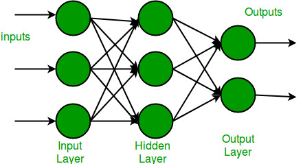
- Input Layer:
- This layer receives raw data as input.
- Each neuron corresponds to a feature in the dataset.
- Example: If the dataset has 10 features, the input layer has 10 neurons.
- Hidden Layers:
- These are the intermediate layers between the input and output layers.
- Hidden layers extract complex patterns by learning hierarchical representations.
- Each neuron in a hidden layer applies weights, biases, and an activation function.
- Output Layer:
- This layer provides the final prediction.
- The number of neurons depends on the task:
- Binary classification: 1 neuron with a sigmoid activation.
- Multi-class classification: NN neurons (one for each class) with softmax activation.
- Regression: 1 neuron with a linear activation.
Fully Connected Structure
Each neuron in one layer is connected to every neuron in the next layer. This is called a fully connected (dense) network, represented mathematically as:
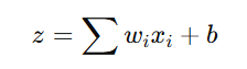
where:
- wi are the weights that adjust the importance of inputs.
- xi are the inputs from the previous layer.
- b is the bias term that helps in shifting the activation function.
- z is the computed weighted sum before applying activation.
Activation Functions in MLP
MLPs use non-linear activation functions to enable the network to model complex relationships. Some commonly used activation functions are:
1. Sigmoid Activation
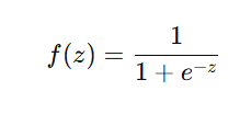
- Output range: (0,1)
- Used in binary classification problems.
- Limitations:
- Vanishing gradient problem: Small gradients slow down learning in deep networks.
2. ReLU (Rectified Linear Unit)
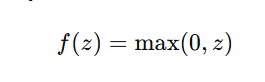
- Output range: [0, ∞)
- Most commonly used activation in deep networks.
- Advantages:
- Solves the vanishing gradient problem.
- Efficient computation.
- Limitations:
- Dying ReLU problem: Neurons may get stuck at 0 if gradients vanish.
3. Softmax Activation
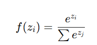
- Converts raw scores into probabilities for multi-class classification.
- Ensures that all outputs sum to 1.
4. Tanh Activation
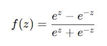
- Output range: (-1,1)
- Better than sigmoid as it centers data around zero.
- Still suffers from vanishing gradient in deep networks.
Training Process of MLP
Training an MLP involves adjusting weights and biases to minimize the error in predictions. This is done using forward propagation, backpropagation, and optimization.
1. Forward Propagation
- Inputs pass through the network layer by layer.
- Each neuron computes a weighted sum and applies an activation function.
- The output layer produces the final prediction.
2. Loss Function Calculation
A loss function measures how far the predicted output is from the actual value.
Common Loss Functions:
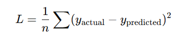
- Mean Squared Error (MSE) – Used for regression problems:
- Cross-Entropy Loss – Used for classification problems:

3. Backpropagation and Weight Updates
- The error is propagated backward to adjust weights using gradient descent.
Weight updates follow:
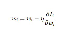
where:
- η is the learning rate.
- ∂L/∂Wi is the gradient of loss w.r.t. weights.
4. Optimization Techniques
To improve training efficiency and prevent overfitting, various techniques are used:
- Gradient Descent Variants:
- Stochastic Gradient Descent (SGD): Updates weights after each sample.
- Mini-batch Gradient Descent: Updates weights after small batches.
- Adam Optimizer: Combines momentum and adaptive learning rates.
- Regularization Techniques:
- L1/L2 Regularization: Prevents overfitting by adding weight penalties.
- Dropout: Randomly drops neurons to force the model to learn robust features.
- Batch Normalization: Normalizes activations to stabilize training.
Advantages of MLP
- Solves non-linear problems (e.g., XOR problem).
- Capable of deep learning when stacked with more layers.
- Universal Approximation Theorem: Can approximate any continuous function.
- Supports both classification and regression tasks.
Applications of MLP
MLPs are widely used in various domains:
1. Computer Vision
- Handwriting Recognition: Used in Optical Character Recognition (OCR).
- Facial Recognition: Identifies faces in security systems.
2. Speech and Audio Processing
- Speech Recognition: Converts spoken language into text (e.g., Siri, Google Assistant).
- Music Genre Classification: Identifies genres from audio signals.
3. Finance and Business
- Stock Market Prediction: Forecasts stock prices using historical data.
- Fraud Detection: Identifies fraudulent transactions.
4. Healthcare and Medicine
- Medical Diagnosis: Detects diseases from medical images (e.g., cancer detection).
- Drug Discovery: Helps in predicting drug interactions.
5. Natural Language Processing (NLP)
- Spam Detection: Filters spam emails.
- Sentiment Analysis: Determines emotions in text.
Comparison Between Perceptron and MLP
| Feature | Perceptron | Multi-Layer Perceptron (MLP) |
|---|---|---|
| Number of Layers | Single-layer | Multiple layers (input, hidden, output) |
| Problem Solving | Only linear problems | Solves both linear and non-linear problems |
| Activation Function | Step function | Sigmoid, ReLU, Softmax, etc. |
| Training Algorithm | Perceptron learning rule | Backpropagation + Gradient Descent |
| Real-World Applications | Simple classification tasks | Image recognition, NLP, fraud detection |
Key Takeaways of Multi-Layer Perceptron (MLP)
- MLP is a type of Artificial Neural Network (ANN) that consists of multiple layers (input, hidden, and output) and is used for solving complex problems.
- Uses fully connected layers, where each neuron in one layer connects to every neuron in the next.
- Activation functions like ReLU, Sigmoid, Softmax, and Tanh enable non-linearity, allowing MLPs to learn complex patterns.
- Training involves forward propagation, loss calculation, and backpropagation, using gradient descent to update weights.
- Optimization techniques like Adam, SGD, dropout, and batch normalization improve learning efficiency and prevent overfitting.
- MLP is versatile, supporting classification, regression, and function approximation.
- Applications include image recognition, speech processing, finance, healthcare, and NLP.
- Compared to a single-layer perceptron, MLP can solve both linear and non-linear problems using advanced activation functions and backpropagation.
Next Blog- Activation Functions in Deep Learning
.png)
.png)
.png)
.png)
.png)
.png)
.png)
.png)
.png)
.png)
.png)
.png)
.png)
.png)