What Are Deep Q Networks?

Deep Q Networks are an extension of the traditional Q-learning algorithm. They incorporate deep neural networks to approximate the Q-value function, which maps state-action pairs to expected rewards. This approach is particularly useful in environments where the state space is large or continuous, making a tabular representation of Q-values impractical.

Key Concepts:

• Q-Learning Recap:
  Q-learning is a model-free reinforcement learning algorithm that estimates the value of taking a given action in a given state. The core update rule is:

  

  where α is the learning rate, γ is the discount factor, and r is the reward received.

• Deep Learning Integration:
  Instead of maintaining a Q-table, DQNs use a deep neural network to approximate the Q-function. This allows the algorithm to handle high-dimensional inputs such as images or sensor data.

How Do Deep Q Networks Work?

Deep Q Networks (DQNs) combine the power of deep learning with the foundational ideas of Q-learning to handle complex environments with high-dimensional state spaces. Here’s an in-depth explanation of how DQNs work, covering the neural network architecture, experience replay, target networks, and the optimization process.

1. Neural Network Architecture

At the core of a DQN is a deep neural network designed to approximate the Q-value function, which predicts the expected future rewards for each possible action in a given state. Let’s break down the architecture:

Input Layer

• State Representation:
  The input to the network represents the current state of the environment. In many applications, this could be raw pixel data (like in Atari games), sensor readings from a robot, or any other form of structured data that captures the state.
• Preprocessing:
  Often, raw inputs are preprocessed (e.g., normalized, resized) to ensure that the neural network can learn efficiently from them.

Hidden Layers

• Feature Extraction:
  The hidden layers consist of multiple layers of neurons that learn to extract and transform features from the raw input. In the case of image data, convolutional layers might be used to capture spatial hierarchies.
• Non-Linearity:
  Activation functions such as ReLU (Rectified Linear Unit) introduce non-linearity, allowing the network to learn complex mappings between states and Q-values.
• Depth and Complexity:
  The number of layers and the number of neurons in each layer determine the complexity of the model. A deeper network can capture more intricate patterns but may also require more data and computational resources.

Output Layer

• Action Value Predictions:
  The final layer of the network outputs a vector of Q-values—one for each possible action. For example, in a game environment, if the agent has four possible actions (left, right, up, down), the network will output four Q-values corresponding to each action.
• Interpretation:
  These Q-values represent the expected cumulative future reward when taking a specific action in the current state and then following the optimal policy thereafter.

2. Experience Replay

One of the major innovations that made DQNs practical is the introduction of experience replay. This mechanism addresses the issue of correlated data, which can destabilize training.

Memory Buffer

• Storing Experiences:
  As the agent interacts with the environment, each experience is recorded as a tuple (s,a,r,s′)(s, a, r, s'). Here, ss is the current state, aa is the action taken, rr is the reward received, and s′s' is the resulting state.
• Replay Buffer:
  These experiences are stored in a replay buffer (or memory). The buffer holds a large number of past experiences, enabling the network to learn from a diverse set of data points.

Random Sampling

• Breaking Correlations:
  During training, instead of using consecutive experiences (which are likely to be correlated), the agent randomly samples mini-batches from the replay buffer. This randomization breaks the temporal correlations and makes the training data more independent and identically distributed (i.i.d.).
• Stability and Efficiency:
  By training on these random mini-batches, the learning process becomes more stable, and the agent can learn a more robust policy. Additionally, reusing past experiences improves data efficiency.

3. Target Network

DQNs also leverage a target network to improve the stability of the learning process. This technique helps decouple the target Q-value calculation from the rapidly changing Q-network.

Stability in Learning

• Separate Target Calculation:
  Instead of using the same network to estimate both the current Q-values and the target Q-values, a separate target network is maintained. This network has the same architecture as the primary (or online) Q-network but with a set of weights that are updated less frequently.
• Periodic Updates:
  Every few thousand steps (or episodes), the weights of the target network are updated to match those of the online network. This means that while the online network is continuously learning and changing, the target network remains stable for a period, reducing the risk of oscillations or divergence during training.

Decoupling the Target

• Reducing Feedback Loops:
  By using a target network, the Q-value targets used in the loss function remain relatively constant for short periods. This decoupling prevents the feedback loop where the network’s own predictions could quickly shift and destabilize the learning process.
• Convergence:
  With a stable target, the network can more effectively minimize the loss between predicted Q-values and the target Q-values, leading to more reliable convergence over time.

4. Loss Function and Optimization

The goal of training a DQN is to minimize the difference between the predicted Q-values from the neural network and the target Q-values derived from the Bellman equation. This process is carried out using a loss function and optimization techniques.

Loss Function

• Bellman Equation and Target Q-Values:
  DQNs are based on Q-learning, which relies on the Bellman equation to update the Q-values. The Bellman equation for Q-learning is:

  

  where:

• Q(s,a) is the predicted Q-value for taking action a in state s.
• r is the reward received after taking action a.
• s′ is the next state the agent transitions to.
• γ is the discount factor, which determines how much future rewards are valued.
• max⁡a′Q(s′,a′)  is the highest predicted Q-value for the next state s′, meaning the best future reward expected.
• Since a neural network is used to approximate Q(s,a), we need a way to minimize the difference between the predicted Q-values and the target values.

DQN Loss Function

The loss function in a DQN is typically the Mean Squared Error (MSE) between the predicted Q-values and the target Q-values.

where:

• L(θ) is the loss function that we aim to minimize.
• Q(s,a;θ) is the predicted Q-value from the neural network, where θ represents the model parameters.

• y is the target Q-value computed as:

  

  θ− are the weights of the target network, which is a separate copy of the Q-network that updates periodically.

  Intuition Behind the Loss Function

• The loss function measures how far off the predicted Q-value is from the target Q-value:
• If the predicted Q-value is close to the target Q-value:
  • The loss is small, meaning the network is already making good predictions.
  • The model receives a small gradient update.
• If the predicted Q-value is far from the target Q-value:
  • The loss is large, indicating the model needs to adjust its weights.
  • The model receives a larger gradient update to correct the predictions.
• The Mean Squared Error (MSE) is used because it penalizes large differences between predicted and target values, forcing the network to learn accurate Q-values over time.

Training Process: Gradient Descent and Optimization

Once the loss function is defined, we use gradient descent (or its variants like Adam or RMSProp) to update the neural network’s weights.

Gradient Descent Updates

1. Compute the loss L(θ).
2. Calculate the gradient of the loss with respect to the network’s weights θ.
3. Adjust the weights using an optimization algorithm to minimize the loss.

where:

• α is the learning rate (step size).
• ∇L(θ) is the gradient of the loss function with respect to the weights.

Role of the Target Network in the Loss Function

One issue in Q-learning is that the target Q-values keep changing as the network updates. If the targets change too quickly, training becomes unstable.

To solve this, DQNs use a target network Q(s,a;θ−)that is updated only periodically, reducing the risk of unstable learning.

The target Q-values are computed using the target network:

The predicted Q-values are computed using the main (online) network:

The loss function minimizes the difference between these two values.

Example Calculation

Given:

• Current state s: "Player is at position X"
• Action a: "Move right"
• Reward r: +1 (for moving closer to the goal)
• Next state s′: "Player is at position X+1"
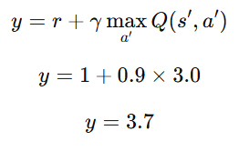
• Discount factor γ: 0.9
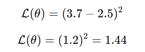
• Predicted Q-value from the online network Q(s,a)=2.5

• Target network estimates max⁡ a′Q(s′,a′)=3.0

  Target Q-value Calculation

  

  Loss Calculation

  

• This loss value is then used to adjust the network weights using gradient descent.

Benefits of Using Deep Q Networks

• Scalability: DQNs can handle complex environments with high-dimensional state spaces, such as video games or robotics.
• Efficiency: Through experience replay and target networks, DQNs achieve faster and more stable convergence compared to traditional Q-learning.
• Flexibility: They can be applied to a wide range of tasks from simple grid worlds to complex simulations.

Practical Applications of DQNs

Deep Q Networks have been successfully applied in various domains:

1. Gaming and Entertainment

• Atari Games: The original breakthrough of DQNs was demonstrated on Atari 2600 games, where the algorithm learned to play directly from raw pixels.
• Esports: Advanced reinforcement learning techniques are now being used to develop AI opponents in competitive gaming.

2. Robotics

• Autonomous Navigation: DQNs help robots learn to navigate environments by interpreting sensor data and making real-time decisions.
• Manipulation Tasks: From grasping objects to performing complex assembly operations, DQNs enhance robot adaptability.

3. Autonomous Vehicles

• Decision Making: In self-driving cars, DQNs are used to make decisions such as lane changing, obstacle avoidance, and speed regulation.
• Simulation Training: They enable extensive simulation training, reducing the need for costly real-world testing.

Key Takeaways

1. Extension of Q-Learning – DQNs improve traditional Q-learning by using deep neural networks to approximate Q-values, enabling learning in complex environments with large state spaces.
2. Neural Network-Based Q-Function – Instead of a Q-table, DQNs use a deep neural network to estimate action values, making them effective for high-dimensional inputs like images.
3. Experience Replay – Stores past experiences in a memory buffer and samples them randomly to break correlations, stabilizing training and improving learning efficiency.
4. Target Network – A separate, periodically updated network reduces training instability by keeping target Q-values stable over short periods.
5. Loss Function & Optimization – Uses the Bellman equation to compute target Q-values and applies Mean Squared Error (MSE) loss with gradient descent-based optimization (e.g., Adam, RMSProp).
6. Scalability & Efficiency – DQNs are more stable and scalable than traditional Q-learning, thanks to techniques like experience replay and target networks.
7. Applications – Used in gaming (Atari, esports AI), robotics (navigation, object manipulation), and autonomous vehicles (decision-making, obstacle avoidance).
   
   Next Blog- Python implementation of Deep Q-Networks (DQN)