Optimization Techniques in Machine Learning

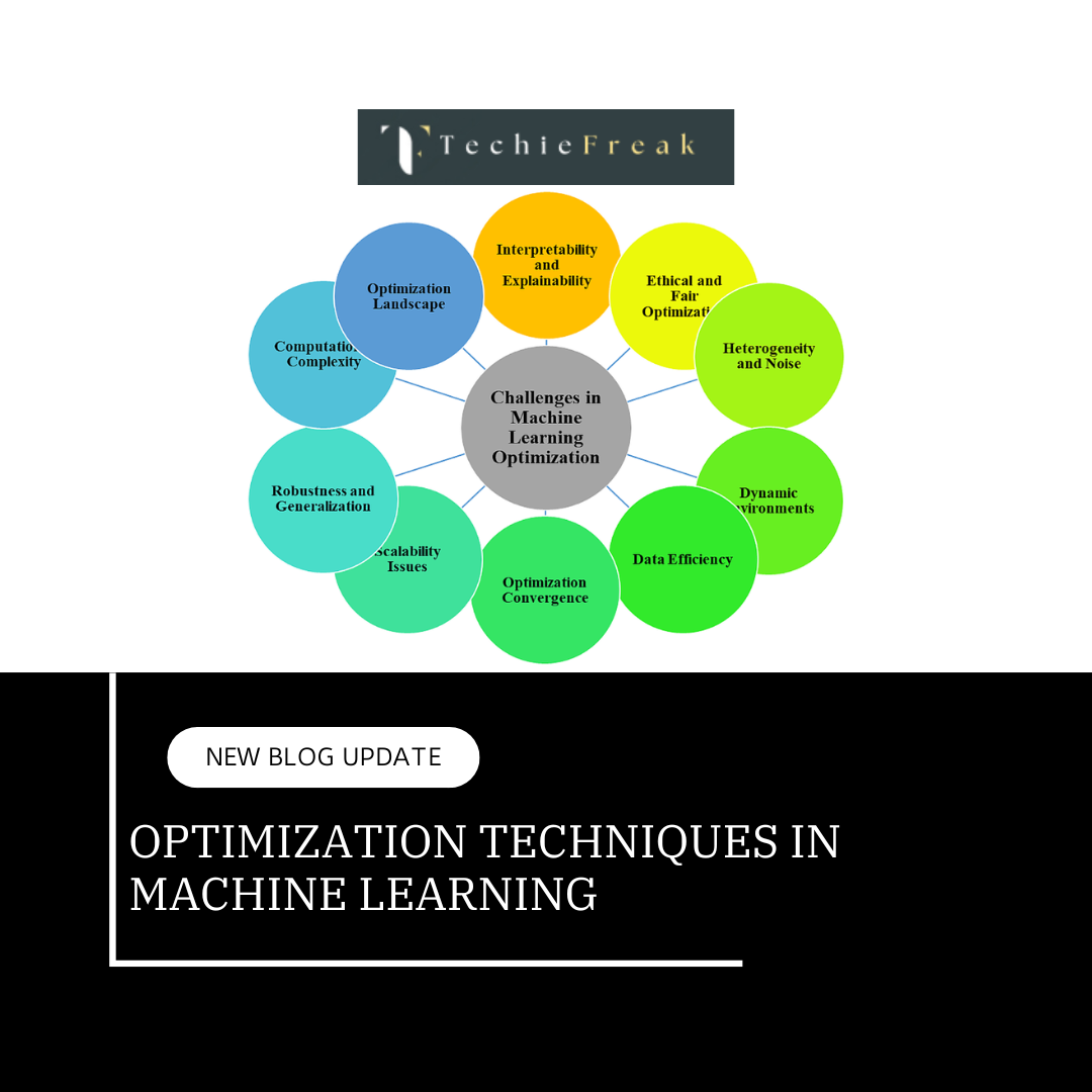
Optimization lies at the core of machine learning. It is the mathematical process by which models adjust their parameters to improve performance, typically by minimizing a loss function. This detailed blog explores key optimization techniques, their principles, strengths, challenges, and practical applications in machine learning workflows.

What is Optimization?

In machine learning, optimization is the process of finding the best set of parameters for a model such that a specific objective or loss function is minimized (or maximized). This objective function quantifies the model's performance, such as the prediction error or the classification loss. The process is iterative and involves fine-tuning the model weights to make accurate predictions on unseen data.

Key Terms:

Here’s an expanded explanation of the key terms:

Objective Function

The objective function represents the ultimate goal of the optimization process in machine learning. It is the mathematical expression that the algorithm seeks to minimize or maximize. For instance:

• In regression problems, the objective function is often Mean Squared Error (MSE), which quantifies how far predictions are from actual values.
• In classification problems, it might be Log-Loss or Cross-Entropy, measuring the accuracy of predicted probabilities.
  Think of it as the "scorecard" for your model—lower or higher values indicate better or worse performance, depending on the context.

Parameters

Parameters are the variables that the optimization algorithm adjusts during training to achieve the best results.

• For example, in a neural network, these are the weights and biases associated with each connection and neuron.
• The optimizer tunes these parameters iteratively to reduce (or increase) the value of the objective function.

Parameters directly influence the model's predictions. Properly optimized parameters ensure that the model can generalize well to new, unseen data.

Learning Rate (η)

The learning rate determines the size of the steps the optimizer takes during the parameter update process. It is a hyperparameter with critical implications for training:

• A large learning rate may result in overshooting the optimal solution, causing instability or divergence.
• A small learning rate makes the training process slow and could potentially get stuck in a local minimum.
  Finding the right balance is crucial for efficient optimization. Advanced techniques like learning rate schedules or adaptive learning rates (e.g., used in Adam or RMSprop) can adjust this dynamically.

Optimization algorithms are critical for two main reasons:

1. They enable the efficient training of machine learning models.
2. They improve generalization, ensuring the model performs well on unseen data.

Optimization Techniques

1. Gradient Descent (GD)

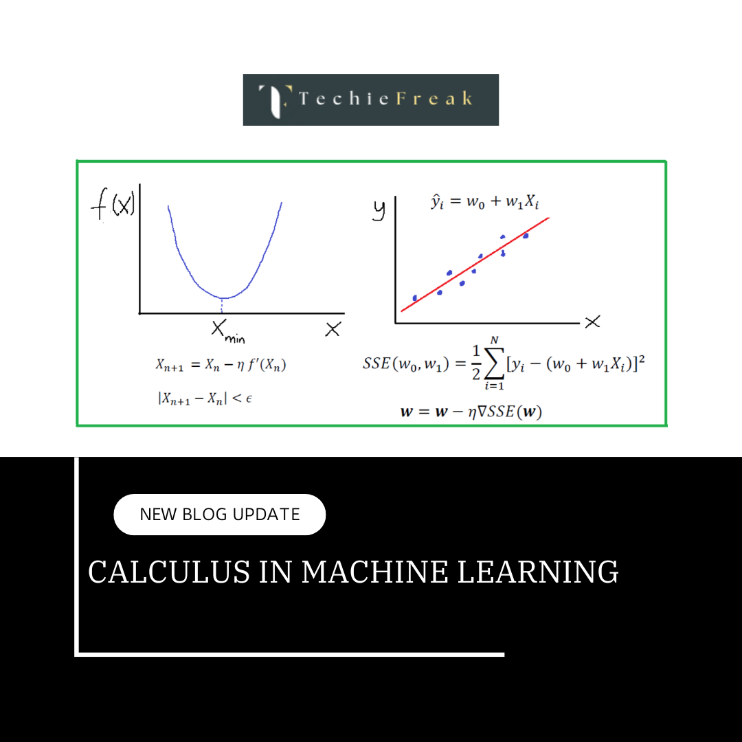
Gradient Descent is the cornerstone of optimization in machine learning. It aims to minimize the loss function by iteratively adjusting the parameters in the opposite direction of the gradient.

Steps in Gradient Descent:

1. Initialize model parameters (e.g., weights, biases) randomly or using specific heuristics.
2. Compute the loss using the current parameters.
3. Calculate the gradient of the loss function with respect to the parameters.

4. Update the parameters using the formula: 

   

5. Repeat until the loss converges to a minimum.

Key Insights:

• Learning Rate (η): Determines the size of each step. A small η\eta leads to slow convergence, while a large η may cause overshooting or divergence.
• Convergence: Achieved when the loss function reaches a stable minimum or when successive updates become negligible.

Variants of Gradient Descent:

• Batch Gradient Descent: Uses the entire dataset for each gradient update. While stable, it is computationally expensive for large datasets.
• Stochastic Gradient Descent (SGD): Updates parameters using one data point at a time, making it faster but noisier.
• Mini-batch Gradient Descent: Balances efficiency and stability by using small subsets (mini-batches) of data for updates.

Applications:

• Training linear regression, logistic regression, and deep neural networks.

2. Stochastic Gradient Descent (SGD)

SGD introduces randomness to the gradient descent process by updating parameters using one training example per iteration.

Advantages:

• Faster convergence for large datasets since it requires less computation per update.
• Inherent noise helps escape saddle points and local minima, particularly useful in non-convex problems.

Challenges:

• High variance in parameter updates leads to fluctuating loss.
• Requires techniques like learning rate schedules, momentum, or averaging to stabilize convergence.

Implementation Example:

# Pseudocode for SGD
for epoch in range(num_epochs):
    for x_i, y_i in training_data:
        gradient = compute_gradient(x_i, y_i, parameters)
        parameters -= learning_rate * gradient

3. Momentum

Momentum improves upon gradient descent by introducing a velocity term to the parameter updates, allowing the algorithm to gain speed in the relevant direction and reduce oscillations.

Update Rule:

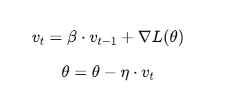
• vt: Velocity term.
• β: Momentum coefficient (commonly set to 0.9).
• ∇L(θ): Gradient of the loss function.

Advantages:

• Accelerates convergence in directions with consistent gradients.
• Reduces oscillations in high-curvature regions.

Applications:

• Commonly used in training deep neural networks to improve convergence speed.

4. RMSProp (Root Mean Square Propagation)

RMSProp adjusts the learning rate for each parameter dynamically based on recent gradient magnitudes, making it suitable for non-stationary objectives.

Update Rule:

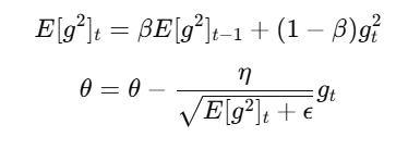
• E[g2]t: Running average of squared gradients.
• ϵ: Smoothing term to prevent division by zero.

Advantages:

• Handles vanishing/exploding gradients effectively.
• Suitable for optimizing deep learning models with complex error surfaces.

5. Adam (Adaptive Moment Estimation)

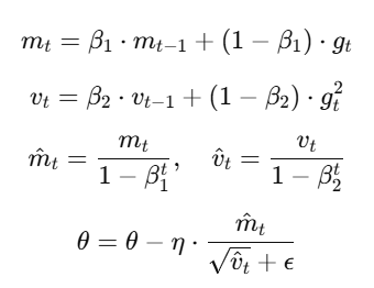
Adam is one of the most popular optimization algorithms due to its robust performance across a wide range of problems. It combines momentum and RMSProp to compute adaptive learning rates for each parameter.

Key Formulas:

Advantages:

• Combines the benefits of momentum and RMSProp.
• Performs well out-of-the-box with minimal hyperparameter tuning.

Disadvantages:

• Requires more memory to store momentum and variance estimates.
• May converge to suboptimal solutions in some cases.

Applications:

• Training deep learning models in frameworks like TensorFlow and PyTorch.

6. Newton’s Method

Newton's Method uses second-order derivatives (Hessian matrix) to find the minima of the loss function. It is particularly effective for convex optimization problems.

Update Rule:

• H: Hessian matrix (second derivative of the loss function).

Advantages:

• Faster convergence for convex loss functions.
• Requires fewer iterations than first-order methods.

Disadvantages:

• Computationally expensive for high-dimensional problems.
• Infeasible for non-convex loss functions or large-scale datasets.

Practical Considerations

When choosing an optimization technique:

1. Problem Type: For deep learning, Adam or RMSProp are often preferred. For simpler models, gradient descent variants suffice.
2. Computational Resources: Use computationally lighter methods like SGD for large datasets.
3. Learning Rate Tuning: Employ learning rate schedules or adaptive techniques to enhance convergence.

Key takeaways:

Optimization techniques are the backbone of machine learning, directly influencing the efficiency and accuracy of models. Understanding the nuances of each method and selecting the right one for your application is critical for success. By experimenting and fine-tuning, machine learning practitioners can unlock the full potential of their models, ensuring robust and reliable performance.

By this we will end our journey for understanding Basic Maths required for Machine Learning.

Now we will move ahead and Master the Machine Learning Algorithms. 

Next Topic : Data Preprocessing