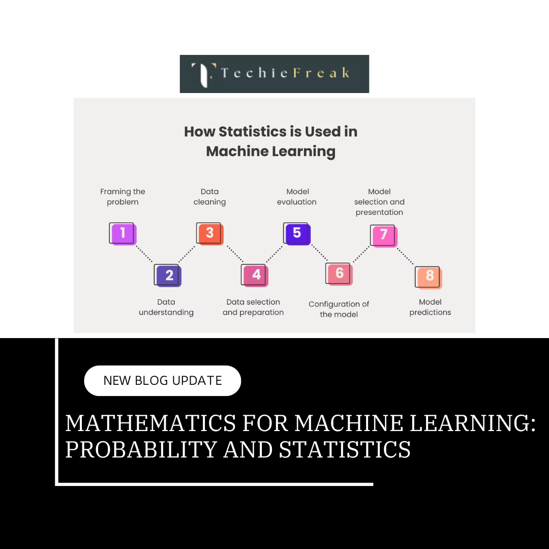
Mathematics for Machine Learning: Probability and Statistics
In the world of machine learning (ML), mathematics serves as the backbone for algorithms, optimization techniques, and decision-making processes. Among various mathematical disciplines, probability and statistics play a pivotal role in enabling machines to learn from data, make predictions, and handle uncertainties. This blog delves into the foundational principles of probability and statistics and explores their applications in machine learning.
Why Probability and Statistics Matter in Machine Learning
Machine learning algorithms often operate in uncertain environments and deal with incomplete or noisy data. Probability provides a framework for modeling uncertainty and randomness, while statistics offers tools to infer insights from data. Together, they enable ML models to:
- Quantify Uncertainty: Handle incomplete data and make probabilistic predictions.
- Generalize from Data: Understand patterns and make inferences about the population from a sample.
- Optimize Models: Use probabilistic models like Bayesian inference for updating beliefs.
- Validate Models: Use statistical tests and metrics to evaluate model performance.
Certainly! Let me expand on each of these sections for better understanding and elaboration:
1. Probability: The Foundation of Uncertainty
Probability serves as the backbone of statistics and data science, quantifying how likely events are to occur.
1.1 What is Probability?
Definition: Probability measures the chance of an event happening, expressed as a value between 0 and 1, where:
- 0 means the event is impossible.
- 1 means the event is certain.
Formula:
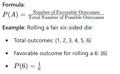
Example: Rolling a fair six-sided die:
- Total outcomes: {1, 2, 3, 4, 5, 6}
- Favorable outcome for rolling a 6: {6}
P(6)=16P(6) = \frac{1}{6}
1.2 Key Concepts and Terminologies
- Experiment: Any process that produces uncertain results.
Example: Tossing a coin, rolling dice, or drawing a card. Sample Space (S): The complete set of all possible outcomes of an experiment.
Example: Tossing a coin results in
Event (A): A subset of the sample space.
Example: For the coin toss,
1.3 Probability Rules
Addition Rule (for union of events):

Explanation: Ensures overlapping probabilities of this are not double-counted.

Example: Drawing a card that is either a heart (H) or a face card (F) from a standard deck:
_1735643449.png)
Multiplication Rule (for intersection of events):

Explanation: The probability of both A and B occurring depends on the probability of A and the conditional probability of B given A.
Complement Rule:

Explanation: The complement A^c represents all outcomes where A does not occur.
1.4 Types of Probability
- Theoretical Probability: Derived from a logical approach without actual trials.
Example: Flipping a fair coin; P(Heads)=0.5 - Empirical Probability: Based on experiments or observed data.
Example: If a coin is flipped 100 times, and Heads appears 60 times, P(Heads)=0.6 - Subjective Probability: Based on intuition or personal belief.
Example: "There’s an 80% chance it will rain tomorrow based on how the sky looks."
1.5 Random Variables
A random variable is a numerical description of the outcomes of a random experiment. It can be classified into two types: discrete and continuous, based on the type of values they can take.
1. Discrete Random Variables
These variables can take on a finite or countable number of distinct values. Each value corresponds to a specific outcome of a random event.
Key Features:
- Values are separate and distinct (no in-between values).
- Commonly used for scenarios involving counting.
Example:
Consider tossing a coin 10 times and counting the number of heads:
- Possible outcomes are whole numbers: 0, 1, 2, ..., 10.
- Each outcome has an associated probability (e.g., P(Number of heads = 5)).
2. Continuous Random Variables
These variables can take on any value within a continuous range. Outcomes are not countable but instead represent measurements.
Key Features:
- Values are infinitely divisible within the range (e.g., decimals or fractions).
- Commonly used for scenarios involving measurement.
Example:
Consider the heights of students in a class:
- Heights can range from, say, 4.5 feet to 6.5 feet.
- Possible values include decimals like 5.1, 5.35, etc.
- Since the range is continuous, the probability of an exact value (e.g., height = 5.0) is effectively zero. Instead, probabilities are calculated over intervals (e.g., P(Height between 5.0 and 5.5)).
Summary Table:
| Type | Values | Examples |
|---|---|---|
| Discrete | Countable, distinct | Number of heads in coin tosses, dice rolls |
| Continuous | Any value in a range | Heights of students, time to complete a task |
Understanding these differences is fundamental to working with probability distributions and analyzing data effectively in machine learning.
1.6 Probability Distributions
A probability distribution describes how the values of a random variable are distributed. It provides a function or table that assigns probabilities to the possible values of a random variable. Probability distributions can be classified into two main types based on the nature of the random variable: discrete and continuous.
Discrete Distributions:
Discrete probability distributions deal with discrete random variables, which take distinct, separate values (like integers). These distributions assign probabilities to each possible value of the variable.
Binomial Distribution: For nn trials, with probability pp of success in each trial:

Example: Probability of 3 heads in 5 tosses of a fair coin:
_1735643514.png)
Poisson Distribution: Models the occurrence of rare events:

Example: If a website gets 2 clicks per minute (λ=2), the probability of 3 clicks in a minute is:

Continuous Distributions:
Continuous probability distributions deal with continuous random variables, which can take any value within a range. Probabilities are assigned over intervals, as the probability of an exact value is zero.
Normal Distribution: Characterized by mean μ\mu and standard deviation σ\sigma.
Probability density function:
Example: Heights of students, with mean μ = 170 cm and σ = 10 cm.
Key Differences Between Discrete and Continuous Distributions
| Feature | Discrete Distributions | Continuous Distributions |
|---|---|---|
| Type of Variable | Discrete random variables (countable values) | Continuous random variables (any value in range) |
| Probability Assignment | Assigns probabilities to specific values | Assigns probabilities over intervals |
| Examples | Binomial, Poisson | Normal, Exponential |
1.7 Bayes' Theorem
Bayes' Theorem is a fundamental concept in probability theory that helps us update our beliefs or probabilities about an event based on new evidence or information. It allows us to revise the probability of an event occurring, given prior knowledge and new data.
Formula:

Where:
- P(A∣B) is the posterior probability: The probability of event AAA occurring given that event BBB has occurred (what we are trying to find).
- P(B∣A) is the likelihood: The probability of observing event BBB, given that event AAA has occurred.
- P(A is the prior probability: The probability of event AAA occurring before observing event BBB.
- P(B) is the evidence: The overall probability of observing event BBB (which may be influenced by all possible causes).
Example:
- P(A)= 0.3 (Probability of having a disease)
- P(B∣A)=0.7 (Probability of testing positive given disease)
- P(B)=0.4 (Overall probability of testing positive)

Interpretation:
This means that, given a positive test result, the probability that you actually have the disease is 52.5%.
Bayes' Theorem helps us adjust the probability (posterior) based on the initial belief (prior) and the likelihood of the new evidence (the test result). This is especially useful in fields like medical diagnostics, where we frequently need to update our beliefs based on new data or tests.
2. Statistics: Understanding Data
2.1 What is Statistics?
Statistics is a branch of mathematics that deals with the collection, analysis, interpretation, and presentation of data. By transforming raw data into meaningful insights, statistics empowers decision-making in various domains like science, business, healthcare, and social sciences.
2.2 Key Statistical Concepts for Machine Learning
1. Descriptive Statistics
Descriptive statistics provide a concise summary of the key features of a dataset. They give us insights into the central tendency, variability, and distribution of the data. These statistics are essential for understanding the data before diving into more complex analyses.
Key Descriptive Statistics Metrics:
Mean (Average):
- The mean is the sum of all values in the dataset divided by the number of values.
- It represents the central value of the dataset.
Formula:

- Where:
- xi = each data point
- n = number of data points
- Example:
For the dataset [1, 2, 3, 4, 5, 6, 7, 8, 9], the mean is:

Median:
- The median is the middle value of a dataset when the data points are arranged in ascending order.
- If the dataset has an odd number of values, the median is the middle value. If it's even, the median is the average of the two middle values.
- Example:
For the dataset [1, 2, 3, 4, 5, 6, 7, 8, 9], the median is 5, because it’s the middle value. Mode:
- The mode is the value that occurs most frequently in the dataset.
- A dataset can have:
- No mode (if all values are unique),
- One mode (unimodal),
- Multiple modes (bimodal or multimodal).
Example:
For the dataset [1, 2, 3, 4, 4, 5, 6, 7], the mode is 4 because it appears twice, more than any other number.- Variance:
- Variance measures the spread of data points from the mean.
- It is the average of the squared differences from the mean.
Formula:

- Where:
- xi = each data point
- μ = mean of the dataset
- n = number of data points
- A high variance indicates that data points are spread out over a wide range, while a low variance suggests that data points are clustered around the mean.
- Standard Deviation:
- The standard deviation is the square root of the variance. It gives a more interpretable measure of spread in the same unit as the data.
- It tells you how much individual data points deviate from the mean on average.
- Formula:

Example in Python:
Here's how we can calculate the mean, median, and standard deviation using Python and the numpy library:
import numpy as np

# Sample data
data = [1, 2, 3, 4, 5, 6, 7, 8, 9]

# Calculate mean, median, and standard deviation
mean = np.mean(data)
median = np.median(data)
std_dev = np.std(data)

# Output the results
print(f"Mean: {mean}, Median: {median}, Standard Deviation: {std_dev}")
Explanation:
- np.mean(data) calculates the average value (mean).
- np.median(data) finds the middle value when the data is sorted.
- np.std(data) computes the standard deviation, giving a sense of how spread out the data is.
Output:
Mean: 5.0, Median: 5.0, Standard Deviation: 2.581988897471611
2. Probability Distributions
In statistics, a probability distribution describes how the values of a random variable are distributed. These distributions are essential for understanding how data behaves and making predictions. Probability distributions can be classified into two main types: discrete and continuous. Below, we'll explore some of the most commonly used probability distributions: Normal Distribution, Binomial Distribution, and Poisson Distribution.
A. Normal Distribution (Gaussian Distribution)
The Normal Distribution is one of the most fundamental and widely used distributions in statistics. It is a continuous probability distribution and is characterized by its bell-shaped curve that is symmetrical around the mean. This means that data points are more likely to be closer to the mean, with fewer points occurring as you move away from the center.
Key Characteristics:
- Symmetrical: The distribution is perfectly symmetrical, with the left and right halves being mirror images.
- Mean, Median, and Mode: In a normal distribution, these three measures of central tendency are all the same and located at the center of the distribution.
- Defined by two parameters:
- Mean (μ): The central value of the distribution.
- Standard Deviation (σ): The measure of the spread of the data.
Formula (Probability Density Function):

Where:
- x = data point
- μ = mean of the distribution
- σ = standard deviation of the distribution
Example:
The heights of students in a classroom are often assumed to follow a normal distribution, where most students are around the average height, and fewer students are very tall or very short.
B. Binomial Distribution
The Binomial Distribution is a discrete probability distribution that models the number of successes in a fixed number of independent trials, each with the same probability of success. It’s used when an experiment can result in just one of two outcomes: success or failure.
Key Characteristics:
- Fixed Number of Trials (n): The number of trials is predetermined and fixed.
- Binary Outcomes: Each trial has two possible outcomes (success or failure).
- Constant Probability (p): The probability of success remains the same for each trial.
- Independent Trials: The outcome of one trial does not affect the others.
Formula (Probability Mass Function):

Where:
- P(X=k)= Probability of getting exactly kk successes
- n = Total number of trials
- k = Number of successes
- p = Probability of success on a single trial
- (nk)\binom{n}{k} = Binomial coefficient, representing the number of ways to choose kk successes from n trials.
Example:
- If you flip a coin 5 times, the binomial distribution can be used to calculate the probability of getting exactly 3 heads (successes), where the probability of heads on each flip is 0.5.
C. Poisson Distribution
The Poisson Distribution is another discrete probability distribution used to model the occurrence of events within a fixed interval of time or space, when these events occur randomly and independently. The Poisson distribution is particularly useful for modeling rare events.
Key Characteristics:
- Rare Events: It is often used to model rare events that happen at an average rate (λ\lambda) within a fixed interval.
- Constant Rate: Events occur at a constant average rate over time or space.
- Independence: The occurrence of one event does not affect the occurrence of another.
- Discrete Values: The number of events is a non-negative integer (0, 1, 2, ...).
Formula (Probability Mass Function):

Where:
- P(X=k) = Probability of kk events occurring
- λ = Average number of events in the interval
- k = Number of events observed
- e = Euler’s number (approximately 2.718)
Example:
- The number of calls received by a customer service center in an hour might follow a Poisson distribution if, on average, the center receives 2 calls per hour. The Poisson distribution could then model the probability of receiving exactly 3 calls in an hour.
Comparison of the Three Distributions
| Distribution | Type | Key Characteristics | Example |
|---|---|---|---|
| Normal Distribution | Continuous | Symmetrical bell curve; defined by mean and standard deviation | Heights of people, test scores |
| Binomial Distribution | Discrete | Fixed number of trials; binary outcomes (success/failure) | Number of heads in a fixed number of coin flips |
| Poisson Distribution | Discrete | Models rare events; events occur at a constant rate | Number of accidents at an intersection per day |
3. Inferential Statistics
Inferential Statistics: An Overview
Inferential statistics allows us to make generalizations, predictions, or conclusions about a population based on a sample of data. Since it's often impractical or impossible to collect data from an entire population, inferential statistics helps us estimate population parameters and test hypotheses. Key techniques within inferential statistics include Hypothesis Testing, Confidence Intervals, and the p-value.
A. Hypothesis Testing
Hypothesis Testing is a method used to assess the validity of assumptions about a population or dataset. The primary goal is to determine whether there is enough statistical evidence in a sample to support or reject a specific hypothesis.
Key Concepts:
- Null Hypothesis (H₀): The default assumption or statement that there is no effect or no difference in the population. It is what we attempt to disprove or reject.
- Alternative Hypothesis (H₁): The hypothesis that suggests a significant effect or difference in the population.
Steps in Hypothesis Testing:
- Formulate Hypotheses: Define the null hypothesis (H₀) and the alternative hypothesis (H₁).
- Choose Significance Level (α): Commonly set at 0.05, this defines the threshold for rejecting the null hypothesis.
- Select the Test and Calculate the Test Statistic: Depending on the data and hypothesis, different tests are used (e.g., t-test, chi-square test).
- Compare the p-value with α: Based on the test statistic, calculate the p-value.
- If p-value ≤ α: Reject the null hypothesis (support for the alternative hypothesis).
- If p-value > α: Fail to reject the null hypothesis (insufficient evidence).
Example:
If you want to test whether a new drug improves recovery time, the null hypothesis might be that the drug has no effect, while the alternative hypothesis could be that the drug does improve recovery time.
B. Confidence Intervals
A Confidence Interval (CI) is a range of values, derived from a sample statistic, that is likely to contain the true population parameter. The wider the interval, the less precise the estimate; the narrower the interval, the more precise it is.
Key Concepts:
- Confidence Level: The probability that the interval will contain the true population parameter. Common levels are 90%, 95%, and 99%.
- Margin of Error: The amount of random sampling error expected in the estimate.
Example:
Suppose the sample mean income in a city is $45,000, with a margin of error of $1,000, and we want to construct a 95% confidence interval. This means we are 95% confident that the true average income in the population lies between $44,000 and $46,000.
C. p-Value
The p-value is a measure used in hypothesis testing to determine the statistical significance of the results. It tells us the probability of obtaining results at least as extreme as the ones observed, assuming the null hypothesis is true.
Key Concepts:
- p-value ≤ α: The result is statistically significant, and we reject the null hypothesis.
- p-value > α: The result is not statistically significant, and we fail to reject the null hypothesis.
Example:
In a clinical trial, if the p-value is 0.03, it means there is a 3% chance of observing the results (or more extreme ones) if the null hypothesis is true. If the significance level is set at 0.05, the p-value indicates that the results are statistically significant, and we reject the null hypothesis.
Summary of Key Concepts
| Technique | Purpose | Key Concept | Example |
|---|---|---|---|
| Hypothesis Testing | Test the validity of assumptions (H₀ vs. H₁) | Null hypothesis vs. alternative hypothesis | Testing if a new drug improves recovery time |
| Confidence Intervals | Estimate the range in which a population parameter lies | Range of values likely to contain the true parameter | Estimating the average income in a city (e.g., $44,000 to $46,000) |
| p-Value | Determine statistical significance | Probability of observing results under the null hypothesis | p-value of 0.03 indicates significant results |
4. Correlation and CovarianceCorrelation and Covariance: A Deeper Dive
Both correlation and covariance are statistical measures used to assess the relationship between two variables. While they are closely related, they convey different information about how two datasets behave in relation to one another.
A. Correlation
Correlation measures the strength and direction of the linear relationship between two variables. It tells us whether and how strongly pairs of variables are related, and whether this relationship is positive, negative, or non-existent.
Key Features of Correlation:
- Range: Correlation values range from -1 to 1.
- +1 indicates a perfect positive correlation (both variables increase together).
- -1 indicates a perfect negative correlation (as one variable increases, the other decreases).
- 0 indicates no linear correlation (the variables do not have any linear relationship).
- Interpretation:
- Positive Correlation: As one variable increases, the other tends to increase (e.g., height and weight).
- Negative Correlation: As one variable increases, the other tends to decrease (e.g., speed and time taken for a fixed distance).
- No Correlation: No discernible pattern between the variables (e.g., shoe size and IQ).
Example:
In the code snippet you provided:
import numpy as np

x = [1, 2, 3, 4, 5]
y = [2, 4, 6, 8, 10]
correlation = np.corrcoef(x, y)[0, 1]
print(f"Correlation: {correlation}")
Here, x and y have a perfect positive correlation of 1, because as x increases, y increases proportionally (the relationship is linear).
B. Covariance
Covariance measures the direction of the relationship between two variables, but unlike correlation, it doesn't provide any indication of the strength of the relationship. It simply tells us whether the variables tend to vary together (increase/decrease together) or not.
Key Features of Covariance:
- Sign of Covariance:
- Positive Covariance: Both variables tend to increase or decrease together (similar to positive correlation).
- Negative Covariance: When one variable increases, the other decreases (similar to negative correlation).
- Magnitude of Covariance: The magnitude of covariance is dependent on the scale of the variables, making it less interpretable on its own. Unlike correlation, which is standardized (values between -1 and 1), covariance can take any value depending on the scale of the variables.
Example:
In the code snippet you provided:
covariance = np.cov(x, y)[0, 1]
print(f"Covariance: {covariance}")
For x and y, the covariance will also indicate that they have a positive relationship, but the actual value of the covariance depends on the units of x and y, which makes it harder to interpret directly compared to correlation.
Correlation vs. Covariance
| Aspect | Correlation | Covariance |
|---|---|---|
| What it Measures | Strength and direction of the linear relationship between variables | Direction of the relationship between variables |
| Scale | Standardized (-1 to 1) | Non-standardized (depends on the scale of data) |
| Interpretability | Easy to interpret because it's on a fixed scale | Harder to interpret due to variable-dependent magnitude |
| Usefulness | Used to measure the strength of the relationship between variables | Used to see if variables change together (but not how strong the relationship is) |
5. Feature Scaling
Feature scaling is a critical step in data preprocessing that transforms features (variables) to a similar scale or range, ensuring that no single feature dominates the analysis due to its larger magnitude. This is particularly important in machine learning algorithms that are sensitive to the scale of the data, such as those based on distance measures (e.g., KNN, SVM) or gradient-based optimization (e.g., linear regression, neural networks).
The two most commonly used feature scaling techniques are Standardization (Z-Score Normalization) and Min-Max Scaling. Each technique has its advantages and is suited to different types of data and machine learning models.
A. Standardization (Z-Score Normalization)
Standardization scales the data by transforming it into a distribution with a mean of 0 and a standard deviation of 1. The formula for standardization is:

Where:
- X is the original value of the feature.
- μ is the mean of the feature.
- σ is the standard deviation of the feature.
Key Features:
- Mean of 0: After standardization, the feature will have a mean (average) of 0.
- Unit Variance: The standard deviation will be scaled to 1, which means the spread of the data is normalized.
- No Boundaries: Unlike Min-Max scaling, standardized data is not constrained to a fixed range (it could range from negative to positive values).
When to Use Standardization:
- When the data follows a Gaussian (normal) distribution or when outliers are present, as standardization does not bind data to a fixed range and is less sensitive to extreme values.
- Algorithms sensitive to variance (e.g., logistic regression, linear regression, k-means clustering, and neural networks) often perform better with standardized data.
Example:
Consider the feature "age" with a mean of 30 and a standard deviation of 5:
A raw age value of 25 will be standardized as

A raw age value of 35 will be standardized as

B. Min-Max Scaling
Min-Max scaling transforms features by rescaling them to a fixed range, usually [0, 1]. The formula for Min-Max scaling is:

Where:
- X is the original value of the feature.
- Xmin is the minimum value of the feature.
- Xmax is the maximum value of the feature.
Key Features:
- Bounded Range [0, 1]: After Min-Max scaling, all the feature values will be within the range of 0 and 1, which is helpful for some algorithms that assume data is within a specific range.
- Sensitive to Outliers: Since the scaling is based on the minimum and maximum values, outliers can distort the scaled data, causing values to be squeezed into a narrow range.
When to Use Min-Max Scaling:
- When the data does not follow a Gaussian distribution, but is rather uniformly distributed, and you want to bound the values to a specific range (such as [0, 1]).
- Algorithms sensitive to the magnitude of features (like neural networks, decision trees) benefit from Min-Max scaling as it ensures that all features contribute equally to the model.
Example:
Consider the feature "income" with a minimum value of 10,000 and a maximum value of 100,000:
A raw income value of 50,000 will be scaled as

A raw income value of 90,000 will be scaled as

Comparison: Standardization vs. Min-Max Scaling
| Aspect | Standardization | Min-Max Scaling |
|---|---|---|
| Range of Output | Data is transformed to have a mean of 0 and a variance of 1. | Data is scaled to a specific range, usually [0, 1]. |
| Sensitivity to Outliers | Less sensitive to outliers. | Very sensitive to outliers. Extreme values can distort the scale. |
| When to Use | When data is normally distributed or when variance matters. | When you need to bound data within a fixed range. |
| Impact of Outliers | Outliers have less impact because the data is scaled using mean and standard deviation. | Outliers can compress the data into a very narrow range. |
2.3 Advanced Statistical Techniques
1. Bayesian Inference
Bayesian inference updates the probability of a hypothesis as more evidence becomes available. It is foundational in Bayesian networks and probabilistic programming.
2. Principal Component Analysis (PCA)
PCA reduces dimensionality by finding the principal components that explain the
3. Linear Regression
Linear regression models the relationship between a dependent variable and one or more independent variables using a linear equation.
Example:
from sklearn.linear_model import LinearRegression

X = [[1], [2], [3], [4], [5]]
y = [2, 4, 6, 8, 10]
model = LinearRegression().fit(X, y)
print(f"Coefficient: {model.coef_}, Intercept: {model.intercept_}")
2.4 Statistics in Model Evaluation
1. Accuracy, Precision, Recall, and F1-Score
- Accuracy: Correct predictions / Total predictions.
- Precision: True Positives / (True Positives + False Positives).
- Recall: True Positives / (True Positives + False Negatives).
- F1-Score: Harmonic mean of precision and recall.
2. Confusion Matrix
A confusion matrix helps visualize the performance of a classification model. It provides insights into true positives, true negatives, false positives, and false negatives.
3. Cross-Validation
Splits data into training and validation sets multiple times to ensure robust model evaluation. Techniques include k-fold cross-validation and stratified sampling.
2.5 Real-World Applications of Statistics in Machine Learning
- Predictive Analytics:
- Forecasting sales or stock prices using time-series data.
- Natural Language Processing (NLP):
- Understanding and generating human language using probabilistic models like Hidden Markov Models.
- Computer Vision:
- Image classification and object detection using statistical features extracted from pixel data.
- Recommender Systems:
- Suggesting products or content by analyzing user preferences and behaviors.
Key takeaways:
- Probability: Includes random variables, probability distributions (like Gaussian), and Bayes' theorem, all crucial for modeling uncertainty and making predictions in machine learning.
- Statistics: Covers descriptive (mean, variance) and inferential statistics (hypothesis testing), helping in data analysis, model evaluation, and decision-making.
- Applications in Machine Learning: Probability and statistics are used for model evaluation (accuracy, precision) and optimizing algorithms, helping to handle uncertainty and improve performance.
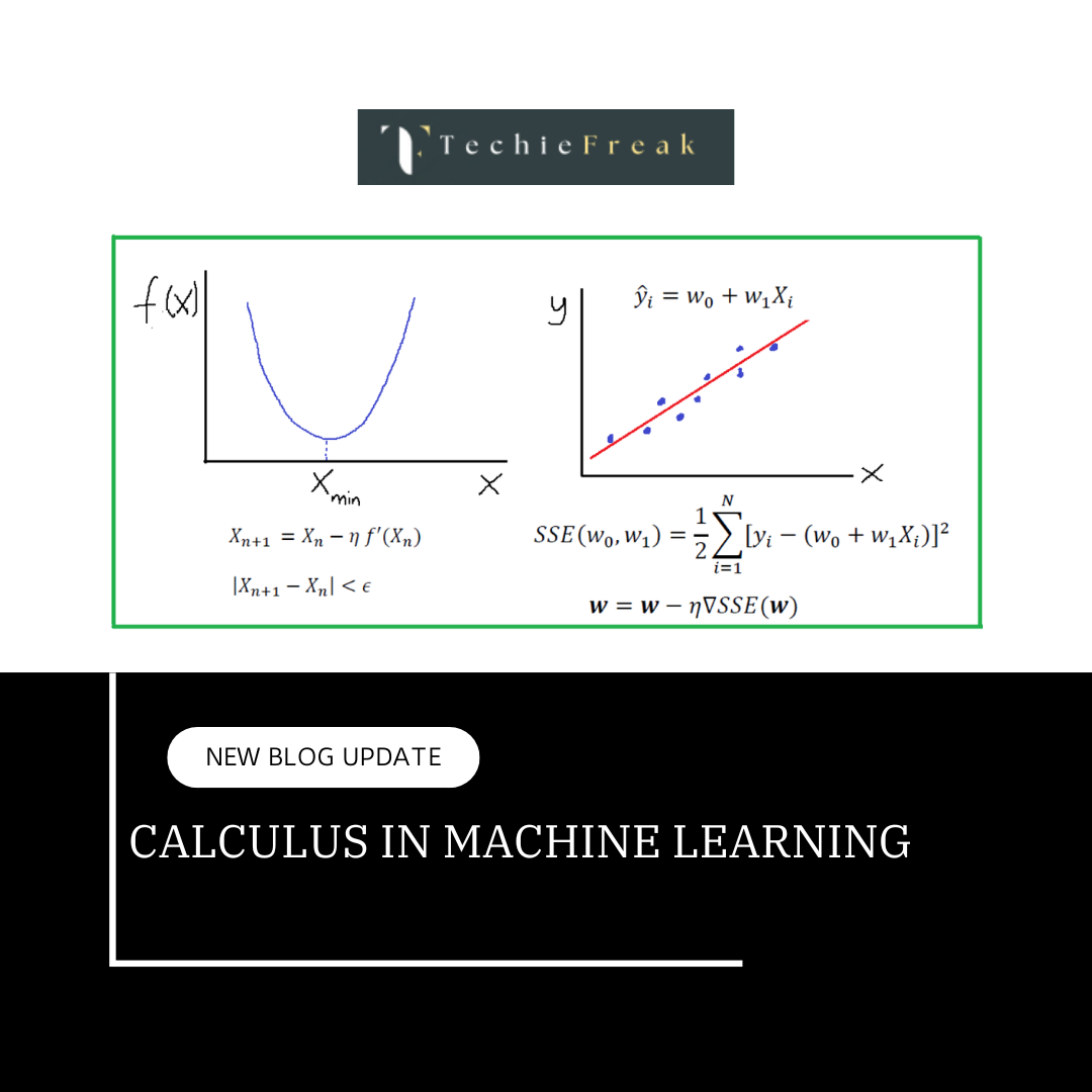
Next Topic : Calculus in Machine Learning
